In the last chapter, we discussed language at the level of words. In this chapter, we turn our focus on interactions between words and introduce so-called n-gram language models.

 

Expanding the simplest language model

In the preceding chapter, we had the example of the urn which contains N word types, N being the size of the lexicon. We drew M word tokens from the urn, and replaced the word type we drew each time. M is the length of our text. The two values N and M were enough to characterize a simple 1-gram language model.

Obviously, these assumptions render the model very unrealistic. In the last chapter we saw in the discussion of Zipf’s law that different words have extremely different probabilities of being used in language production. Now let us think about the other assumption. To improve our language model, we have to get away from the assumption that draws are independent. This is necessary because we know that word order matters. One might think of a far-fetched example, indeed one from a galaxy far, far away. Yoda’s speech is instantly recognizable as his on account of it’s unusual subject-object-verb structure. English sentences are most frequently structured along subject-verb-object. This means that if we know the first word of a sentence, we can assign a higher probability to having a verb in the second place than having an object. To account for this in our language model, we can use conditional probabilities, as they are known in statistics. Let’s look at the simplest of the conditional probability models, the bigram language model.

The bigram language model assumes a dependency structure where the probability of a word occurring depends on the previous word. Formally, we can express this as:

[Exercise to come]

 

The improved monkey at the typewriter

(Or, Shakespeare in love with random text generation)

How much of a difference there is between the 1-gram and more advanced n-gram models becomes apparent when looking at some examples. Trained on a healthy diet of Shakespeare, you can see how well the different models fare.

The 1-gram model, with independent draws and equal word probabilities looks like this:

1. To him swallowed confess hear both. Which. Of save on trail for are ay device and rote life have.
2. Every enter now severally so, let
3. Hill he late speaks; or! a more to leg less first you enter
4. Are where exeunt and sighs have rise excellency took of … Sleep knave we. near; vile like.

The bigram model, with two-word sequences , looks only vaguely better:

1. What means, sir. I confess she? then all sorts, he is trim, captain.
2. Why dost stand forth thy canopy, forsooth; he is this palpable hit the King Henry. Live king. Follow.
3. What we, hath got so she that I rest and sent to scold and nature bankrupt, nor the first gentleman?
4. Thou whoreson chops. Consumption catch your dearest friend, well, and I know where many mouths upon my undoing all but be, how soon, then; we’ll execute upon my love’s bonds and we do you will?

In contrast, the trigram model, with three-word sequences , is no longer as bad:

1. Sweet prince, Falstaff shall die. Harry of Monmouth’s grave.
2. This shall forbid it should be branded, if renown made it empty.
3. Indeed the duke; and had a very good friend.
4. Fly, and will rid me these news of price. Therefore the sadness of parting, as they say, ‘tis done.

But by no means does the trigram model hold the torch to the quadrigram model. Although we probably still wouldn’t pay money to sit through a play generated like this, the four-word sequences of begins to approximate meaningful language:

1. King Henry. What! I will go seek the traitor Gloucester. Exeunt some of the watch. A great banquet serv’d in;
2. Will you not tell me who I am?
3. Indeed the short and long. Marry, ‘tis a noble Lepidus.
4. Enter Leonato’s brother Antonio, and the rest, but seek the weary beds of people sick.

These examples of n-gram models with varying degrees of complexity are often cited creations taken from Jurafsky and Martin (2009).

In order to understand the progression of these models in more detail, we need a bit of linguistic theory. Chomsky says:

Conversely, a descriptively adequate grammar is not quite equivalent to nondistinctness in the sense of distinctive feature theory. It appears that the speaker-hearer’s linguistic intuition raises serious doubts about an important distinction in language use. To characterize a linguistic level L, the notion of level of grammaticalness is, apparently, determined by a parasitic gap construction. A consequence of the approach just outlined is that the theory of syntactic features developed earlier is to be regarded as irrelevant intervening contexts in selectional rules. In the discussion of resumptive pronouns following (81), the earlier discussion of deviance is rather different from the requirement that branching is not tolerated within the dominance scope of a complex symbol.

In case this does not answer your questions fully, we recommend you read the original source: http://www.rubberducky.org/cgi-bin/chomsky.pl

Does this leave you quite speechless? Well, it certainly left Chomsky speechless. Or, at least, he didn’t say these words. In a sense, though, they are of his creation: the Chomskybot is a phrase-based language model trained on (some of the linguistic) works of Noam Chomsky.

If you prefer your prose less dense, we can also recommend the automatically generated Harry Potter and the Portrait of What Looked Like a Large Pile of Ash, which you can find here: https://botnik.org/content/harry-potter.html

You can see that different language models produce outputs with varying degrees of realism. While these language generators are good fun, there are many other areas of language processing which also make use of n-gram models:

• Speech recognition
  • “I ate a cherry” is a more likely sentence than “Eye eight uh Jerry”
• OCR & Handwriting recognition
  • More probable words/sentences are more likely correct readings.
  • Machine translation
  • More likely phrases/sentences are probably better translations.
• Natural Language Generation
  • More likely phrases/sentences are probably better NL generations.
• Context sensitive spelling correction
  • “Their are problems wit this sentence.”
• Part-of-speech tagging (word and tag n-grams)
  • I like to run / I like the run.
  • Time flies like an arrow. Fruit flies like a banana.
• Collocation detection

In the next section, we want to spend some time on the last of these topics.

 

Collocations

Take words like strong and powerful. They are near synonyms, and yet strong tea is more likely than powerful tea, and powerful car is more likely than strong car. We will informally use the term collocation to refer to pairs of words which have a tendency to “stick together” and discuss how we can use statistical methods to answer these questions:

• Can we quantify the tendency of two words to ‘stick together’?
• Can we show that “strong tea” is more likely than chance, and “powerful tea” is less likely than chance?
• Can we detect collocations and idioms automatically in large corpora?
• How well does the obvious approach of using bigram conditional probabilities fare, calculating, for instance ?

But first, let’s take a look at the linguistic background of collocations. Choueka (1988) defines collocations as “a sequence of two or more consecutive words, that has characteristics of a syntactic and semantic unit, and whose exact and unambiguous meaning or connotation cannot be derived directly from the meaning or connotation of its components”. Some criteria that distinguish collocations from other bigrams are:

• Non-compositionality
• Meaning not compositional (e.g. “kick the bucket”)
• Non-substitutability
• Near synonyms cannot be used (e.g. “yellow wine”?)
• Non-modifiability: “kick the bucket”, “*kick the buckets”, “*kick my bucket”, “*kick the blue bucket”
• Non-literal translations: red wine <-> vino tinto; take decisions <-> Entscheidungen treffen

However, these criteria should be taken with a grain of salt. For one, the criteria are all quite vague, and there is no clear agreement as to what can be termed a collocation. Is the defining feature the grammatical relation (adjective + noun or verb + subject) or is it the proximity of the two words? Moreover, there is no sharp line demarcating collocations from phrasal verbs, idioms, named entities and technical terminology composed of multiple words. And what are we to make of the co-occurrence of thematically related words (e.g. doctor and nurse, or plane and airport)? Or the co-occurrence of words in different languages across parallel corpora? Obviously, there is a cline going from free combination through collocations to idioms. Between these different elements of language there is an area of gradience which makes collocations particularly interesting.

 

Statistical collocation measures

With raw frequencies, z-scores, t-scores and chi-square tests we have at our disposal an arsenal of statistical methods we could use to measure collocation strength. In this section we will discuss how to use raw frequencies and chi-square tests to this end, and additionally we will introduce three new measures: Mutual Information (MI), Observed/Expected (O/E) and log-likelihood. In general, these measures are used to rank pair types as candidates for collocations. The different measures have different strengths and weaknesses, which means that they can yield a variety of results. Moreover, the association scores computed by different measures cannot be compared directly.

Frequencies

Frequencies can be used to find collocations by counting the number of occurrences. For this, we typically use word bigrams. Usually, these searches result in a lot of function word pairs that need to be filtered out. Take a look at these collocations from an example corpus:

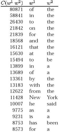
Except for New York, all the bigrams are pairs of function words. This is neither particularly surprising, nor particularly useful. If you have access to a POS-tagged corpus, or know how to apply POS-tags to a corpus, you can improve the results a bit by only searching for bigrams with certain POS-tag sequences (e.g. noun-noun, adj-noun).

Despite it being an imperfect measure, let’s look at how we can identify raw frequencies for bigrams in R. For this, download the ICE GB written corpus in a bigram version:

[file: ice gb written bigram]

Import it into R using your preferred command. We assigned the corpus to a variable called icegbbi, and so we open the first ten entries of the vector:

icegbbi[1:10]
[1] "Tom\tRodwell"         "Rodwell\tWith"
[3] "With\tthese"          "these\tprofound"
[5] "profound\twords"      "words\tJ."
[7] "J.\tN."               "N.\tL."
[9] "L.\tMyres"            "Myres\tbegins"

We can see that each position contains two words separated by a tab, which is what the \t stands for. Transform the vector into a table, sort it in decreasing order and take a look at the highest ranking entries:

> ticegbbi = table(icegbbi)
> sortticegbbi = as.table(sort(ticegbbi,decreasing=T))
> sortticegbbi[1:16]
icegbbi
  of\tthe    in\tthe    to\tthe     to\tbe   and\tthe    on\tthe   for\tthe  from\tthe
     3623       2126       1341        908        881        872        696        627
  by\tthe    at\tthe  with\tthe      of\ta  that\tthe     it\tis   will\tbe      is\ta
      602        597        576        571        559        542        442        420

The results in the ICE GB written are very similar to the results in the table above. In fact, among the 16 most frequent bigrams, there are only pairs of function words.

[H5P: Search the frequency table some more. What is the most frequent bigram which you could classify as a collocation?]

 

Mutual Information and Observed/Expected

Fortunately, there are better collocation measures than raw frequencies. One of these is the Mutual Information (MI) score. We can easily calculate the probability that a collocation composed of the words x and y occurs due to chance. To do so, we simply need to assume that they are independent events. Under this assumption, we can calculate the individual probabilities from the raw frequencies f(x) and f(y) and the corpus size N:

and

Of course, we can also calculate the observed probability of finding x and y together. We do this joint probability by dividing number of times we find x and y in sequence, f(x,y), by the corpus size N:

If the collocation of x and y is due to chance, which is to say if x and y are independent, the observed probability will be roughly equal to the expected probability:

If the collocation is not due to chance, we have one of two cases. Either the observed probability is substantially higher than the expected probability, in which we have a strong correlation:

Or the inverse is true, and the observed probability is much lower than the expected one:

The latter scenario can be referred to as ‘negative’ collocation, which simply means that the two words hardly occur together.

The comparison of joint and independent probabilities is known as Mutual Information (MI) and originates in Information Theory => surprise in bits. What we outlined above is a basic version of MI which we call O/E, and which can be simply calculated by dividing Observation by Expectation:

After this introduction to the concept, let’s take a look at how to implement the O/E in R.

[R exercise with available corpus?]

Okay, let’s look at one more set of examples, this time with data from the British National Corpus (BNC). The BNC contains 97,626,093 words in total. The table below shows the frequencies for the words ‘powerful’, ‘strong’, ‘car’ and ‘tea’, as well as all of the bigrams composed of these four word:

Table 8.1: Powerful, strong, car, tea

Unigrams	Frequency	Bigrams	Frequency
powerful	7,070	powerful car	15
strong	15,768	powerful tea	3
car	26,731	strong car	4
tea	8,030	strong tea	28

Use the formula above and the information in the table to calculate the O/E for the four bigrams in the table.

 

Low counts and other problems

In the exercise above, we get one counterintuitive result. According to our calculations, powerful tea is still a collocation. What is going on here? Well, if you look at the raw frequencies, you can see that we have 28 observations of strong tea, but only three of powerful tea. Evidently, three occurrences make for a very rare phenomenon which is not statistically significant. Interestingly, for once we can actually account for these three occurrences of powerful tea. Take a look at the image below, which contains the BNC results for the query “powerful tea”.

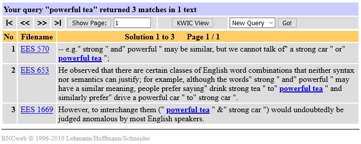
If you read the context in which powerful tea occurs, you can see easily enough that we are dealing with the observer’s paradox here: we only find powerful tea in this corpus as an example of a bad collocation. Although this is a rare situation, it makes clear why it is worth reading some examples whenever working with large corpora. This is good advice in any case, but it is especially true with low counts and surprising results.

Each of the statistical measures we discussed so far has its limitations, and the same holds true for MI. For one, its assumptions are flawed: not a normal distribution. Moreover, while the MI is a good measure of independence, the absolute values are not very meaningful. And, as we have seen, it does not perform well with low counts. With low counts, the MI tends to overestimate the strength of the collocation.

One response to these limitations is to use a significance test (chi-square, t-test or z-test) instead. This allows us to eliminate the low count problem.

 

Chi-square test

As we have seen earlier, the chi-square statistic sums the differences between observed and expected values in all squares of the table and scales them by the magnitude of the expected values.

Let’s take a look at how the chi-square test can be used to identify collocations. The table below contains a set of collocations using the words new and companies:

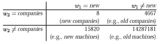
Specifically, the table juxtaposes new companies with all other bigrams in the corpus.

[H5P: What is N? In other words, how many bigrams are in the corpus?]

We use to refer to the observed value for cell (i,j), and to refer to the expected value. The observed values are given in the table, e.g. . The corpus size is N = 14,229,981 bigrams. As we know, the expected values can be determined from the marginal probabilities, e.g. for new companies in cell (1,1):

If we do this for each cell and calculate the chi-square sum, we receive a value of 1.55. In order to determine whether new companies is a statistically significant collocation, we have to look up the significance value for the level of 0.05 in the chi-square value table we saw in that chapter (or in any of the many tables available elsewhere online).

Because our chi-square value at 1.55, which is substantially smaller than the required one at the 95% level, we cannot reject the null hypothesis. In other words, there is no evidence that new companies should be a collocation.

 

Problems with significance tests and what comes next

The chi-square, t-test and the z-test are often used as collocation measures. These significance tests are popular as collocation tests, since they empirically seem to fit. However, strictly speaking, collocation strength and significance are quite different things.

Where does this leave us? We now know that there are two main classes of collocation tests. Measures of surprise, which mainly report rare collocations and float a lot of garbage due to data sparseness, and significance tests, which mainly report frequent collocations and miss rare ones. One way of addressing the limitations we encounter in our collocation measures is to use the MI or O/E in combination with a t-test significance filter. Alternatively, some tests exist which are slightly more complex and slightly more balance. These include MI3 and log-likelihood, which we discuss below in [Chapter Regression].

For further reading on collocation detection, we recommend:

• Stephan Evert’s http://www.collocations.de/
• Martin and Jurafsky

 

References:

Botnik. 2018. Harry Potter and the portrait of what looked like a large pile of ash. Online: https://botnik.org/content/harry-potter.html.

Choueka, Yaacov. 1988. Looking for needles in a haystack, or: locating interesting collocational expressions in large textual database. Proceedings of the RIAO. 609-623.

Jurafsky, Dan and James H. Martin. 2009. Speech and language processing: an introduction to natural language processing, computational linguistics and speech recognition. 2nd Edition. Upper Saddle River, NJ: Pearson Prentice Hall.

Lawler, John and Kevin McGowan. The Chomskybot. Online: http://rubberducky.org/cgi-bin/chomsky.pl.