In this chapter, we discuss logistic regression, a form of regression analysis particularly suited for categorical data.

Introduction to non-linear regression

https://uzh.mediaspace.cast.switch.ch/media/0_ecj2jkhz

In the last chapter, we discussed simple and multiple linear regression without mentioning that one may encounter data where a linear model does not make sense. Let’s look at one of these cases now:

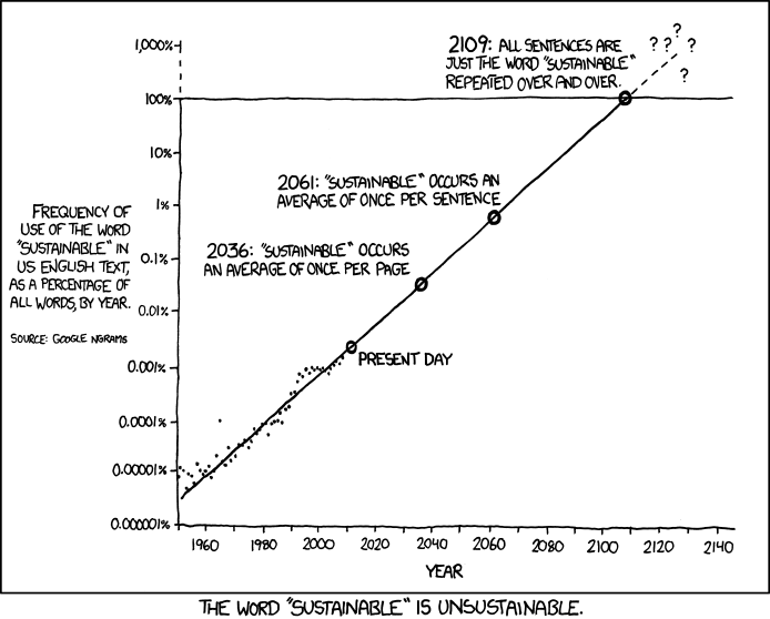
This fantastic comic from xkcd plots a linear model of the frequency of the word ‘sustainable’. We can see that if the trend of the model is correct, English language texts will consist exclusively of the word sustainable by 2109. So while there clearly is a trend to be observed here, the linear model does an abysmal job of capturing it. This is, of course, perfect for the joke here, but it can become a serious issue when trying to analyze data.

A word can be the word “sustainable” only once, then it has reached 100%. It cannot be more than that. If we abstract away from this example, a word can belong to one of several categories corresponding to different lexical items and this is a decision which is taken, and it is nominal. Because these categories are nominal, linear regression, which predicts outcomes on a scale of negative infinity to infinity, no longer makes sense. Instead we need something with which we can make categorical predictions. There are many different types of regression, and some of these provide a solution to the problem of categorical prediction. The table below, from Kabocoff (2011: 175), lists the most common types of regression.

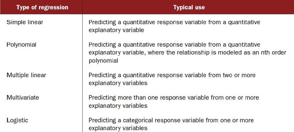
We have already seen simple and multiple linear regressions in action in the last chapter. Additionally, and among others, there is polynomial regression, where we do not model a line but a more complex curve, multivariate regression, where we predict more than one response variable, and logistic regression, with which we can predict categorical outcomes. This is the solution to our problem.

In linguistics, this last type, the logistic regression, is particularly important because very often we are dealing with categories. The example  in the last chapter was passive forms: either a the verb in a sentence is in the active form or it is in the passive form. There is nothing between the two. A word cannot be half “sustainable” and half something else. Either word a is “sustainable” or it is something else. Similarly, in the dative shift, which we discuss below, we cannot have a sentence which begins with “Give…” and continues with a half-prepositional phrase. The sentence is either realized with a noun phrase or with a prepositional phrase. There is no middle ground. This is precisely why logistic regression analysis is particularly important in linguistics.

You will see that the principle of regression analysis which we discussed in the last chapter stays the same with logistic regression, but that things become more complicated. What particularly complicates matters is that in the background of the logistic regression there is a mapping function which maps the numerical output onto a categorial output. For a detailed discussion of this, we recommend reading …. For our part, we are interested in discussing logistic regression not on a technical level, but on a conceptual and practical one.

Motivating logistic regression for linguistic data

https://uzh.mediaspace.cast.switch.ch/media/0_ccoxoxv3

Before we demonstrate the logistic regression properly, we briefly want to scope out the data and point out the inadequacies of the methodologies we discussed so far. We are working here with the ditransitive verbs dataset, which you will remember from chapter one. When we have a ditransitive verb such as ‘give’ or ‘offer’, we have the option of using two noun phrase objects, for instance “give you a book”, or the version where the recipient is realized as a prepositional phrase, such as “give a book to you”. There are many factors which impact the decision of whether the recipient is realized as a noun phrase (NP) or a prepositional phrase (PP), and we can investigate how important these are using logistic regression.

First, though, we should reacquaint ourselves with the dataset. Import the verbs.txt data into R from wherever you stored it (or download it again). We have again opted to name our variable verbs. Let’s take a look at the first few lines:

> head(verbs)
  RealizationOfRec  Verb AnimacyOfRec AnimacyOfTheme LengthOfTheme
1               NP  feed      animate      inanimate      2.639057
2               NP  give      animate      inanimate      1.098612
3               NP  give      animate      inanimate      2.564949
4               NP  give      animate      inanimate      1.609438
5               NP offer      animate      inanimate      1.098612
6               NP  give      animate      inanimate      1.386294

We see that the first column holds the realization of the recipient: this is what we will want to predict. We also see that at the beginning of the table, all recipients are realized as NPs. We can look at the end of the table with the tail() command:

> tail(verbs)
    RealizationOfRec  Verb AnimacyOfRec AnimacyOfTheme LengthOfTheme
898               PP  give      animate      inanimate      1.098612
899               PP  give      animate      inanimate      1.098612
900               PP offer      animate      inanimate      1.791759
901               PP   pay      animate      inanimate      0.000000
902               PP  give      animate      inanimate      1.386294
903               PP  give    inanimate      inanimate      1.098612

This is where all the PPs are.

We can, and should, hypothesize about what factors will impact the realization of the recipient. An invented exampled that sheds some light would be something like the following: “He gave the students who had achieved an extremely remarkable and impressive result in the exam a book”. It is almost impossible to follow sentences where the recipient is a long noun phrase, so we would expect that longer recipients would increase the likelihood of seeing the recipient realized with a prepositional phrase. Other factors – the verb, the animacy of the recipient, the animacy of the theme and the length of the theme – might be just as important. We can look at the trends to develop some intuition for how these factors influence the realization of the recipient.

The first correlation we want to look at is the relationship between the animacy of the recipient and the realization of the recipient. To do this, we can create a contingency table containing these two variables using the xtabs() command:

> tabAnimacyRealiz <- xtabs(~ AnimacyOfRec + RealizationOfRec, data=verbs)

And then we can check out the table:

> tabAnimacyRealiz
            RealizationOfRec
AnimacyOfRec  NP  PP
   animate   521 301
   inanimate  34  47

We see here that there seems to be a clear preference for NP realization of the recipient if the recipient is animate (521>>301), while there seems to be a slight trend towards PP realizations when the recipient is inanimate (34<479).

We can do the same analysis for the length of the theme. Again, we create the appropriate table and look at it:

> tabLengthRealiz <- xtabs(~ LengthOfTheme + RealizationOfRec, data=verbs)
> tabLengthRealiz

In contrast to the previous one, this table is too long for us to get a useful overview which is why we don’t show it. Instead, we want to resort to the familiar chi-square test to reach a better understanding of how the length of the theme relates to the realization of the recipient. Remember that it is best to approach the chi-square test with the hypotheses in mind:

We can run the chi-square test on our table:

>chisq.test(tabLengthRealiz)
	Pearson's Chi-squared test
data:  tabLengthRealiz
X-squared = 144.53, df = 34, p-value = 1.394e-15

The probability value we get for the chi-square test is almost zero, so the pattern we observe in the data for the relationship of the length of theme and the realization of the recipient is clearly non-random. The same holds true for the realization and the animacy of the recipient:

> chisq.test(tabAnimacyRealiz)

If you are asking yourself why this is useful, think about what we just did: we performed two chi-square tests on the relationships between two variables, and in both cases rejected the null hypothesis. In both cases, the null hypothesis stated that there is no meaningful relationship between the two variables. Since we rejected the null hypothesis, we can work with the idea that there is a significant relationship between the two variables. Therefore, we have a reasonable basis to expect that we can predict the realization of the recipient using both the length of the theme and the animacy of the recipient.

Still, there is an important caveat to using the chi-square test in a multi-factor environment such as this: the outcome of the chi-square test (and also of the t-test) is affected if factors other than the one by which we split the data have an important impact on the variable of interest. And this is precisely why we want to analyze our data using a methodology which accounts for multiple explanatory variables at the same time and which is capable of predicting categorical outcomes. This is why we work with the logistic regression.

Logistic regression in R

https://uzh.mediaspace.cast.switch.ch/media/0_jscwtm3w

To frame what we are doing here, you can think about a psycholinguistic situation in which we want to predict whether a speaker will be more likely to use the NP or the PP version. This is precisely what we do when we run a logistic regression in R. To do that, we need the glm() function, which stands for generalized linear model. Unlike the linear model we worked with in the last chapter, the generalized linear model includes the logistic regression. Still, we need to tell R that we want to run a logistic regression, and we do so with the argument family=binomial. This makes it clear to R that we want to use a binomial distribution and run a logistic regression. Of course, we also have to specify the independent variables. For once, we want to condition our model on all available factors, namely the verb, the animacy of the recipient, the animacy of the theme and the length of the theme. Now that we know what we’re doing, we can assign the logistic model to a new variable that we call verbfit:

> verbfit = glm(RealizationOfRec ~ Verb + AnimacyOfRec + AnimacyOfTheme + LengthOfTheme, family = binomial, data = verbs)

That’s it. We have just created a logistic regression model. The real challenge begins with the interpretation. Let’s take a look at the summary:

> summary(verbfit)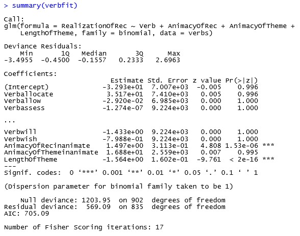

The first thing that becomes obvious is that, because we  have so many different verbs in our data, we have a lot more factors than in any of the models we previously looked at. For aesthetic reasons we decided to abbreviate the list a bit in figure 10.3. What will strike you when you scroll through the list of factors is that none of the verbs is significant predictor for the realization of the recipient. There are no asterisks behind any of the verb coefficients. According to our model, then, the ditransitive verb itself does not impact the realization of the recipient.

Indeed, from this long list of factors only two are significant: the animacy of the recipient and the length of the theme. Both are marked with three asterisks, indicating that they are significant at the 99.9% level. If we look at the probability values, we can see that length of theme is probably more significant for the realization of the recipient than the animacy of the recipient. These probability values from the logistic regression are consistent with the chi-square tests we ran above.

So far, so peachy. But how do we interpret the coefficients? When we discussed linear models, we could readily see how each coefficient contributes to the model. This becomes substantially more difficult with the logistic regression, and we won’t go into the details about why this is the case. Neither will we discuss how to actually interpret the coefficients, since, for linguistic purposes this is hardly ever necessary. Usually, it suffices to understand the significance level and the direction of the effect of a factor. However, for a good discussion of how to interpret the coefficients of logistic models we can recommend the explanation in chapter 13 of Kabacoff (2011).

Even without a precise understanding of how the coefficient of each factor affects the outcome, the logistic regression offers some valuable insights. Firstly, the model tells us which features are significant and which aren’t. Quite often, this is what we are really interested in, since it allows for making claims about which factors contribute to the outcome of interest and which don’t. Secondly, by looking at whether there is a plus or a minus before a coefficient, we can also see at a glance in which direction it pushes the dependent variable. How can we tell?

Well, the default value for animacy of recipient is animate, which we can see by the fact that the third to last row is labelled “AnimacyOfRecinanimate”. The coefficient here is positive, with a value of roughly 1.5. This means that in rows with an inanimate recipient, we have a higher probability of seeing the recipient realized as a PP. Similarly, we can think through the effect of length of theme. Unlike the animacy of the recipient, which is a categorical variable, the length of theme is a continuous variable. Accordingly, we have to think in absolute, continuous numbers rather than categories. What we can say, then, is that an increase in the length of theme results in a lower likelihood of realizing the recipient as a PP.

You may be wondering how we can tell that a positive coefficient increases the probability of a PP realization, rather than an NP realization. Unfortunately, this is not obvious, and indeed Max makes a mistake when discussing this in the video. We discuss how to find the answer to this question after the next section.

Deviance

https://uzh.mediaspace.cast.switch.ch/media/0_t5l843pn

A further aspect of the logistic regression which makes it more complicated than the linear regression is that there is no obvious measure for the quality of a model. Remember that the linear model output came with the R-squared value, which told us how much of the variance in the data is explained by our model. There is no comparable measure for the logistic regression which would tell us at a glance how reliable our model is. Fortunately, there are some ways of determining the quality of our model.

The first of these is the deviance. Take a look at the two rows labelled “Null deviance” and “Residual deviance” in the summary output in figure 10.3. These values correspond to a badness of fit: the higher the deviance, the worse the model performs. The null deviance derives from a model where a single independent variable is used to predict the dependent variable. This single predictor model is known in statistics as a baseline model. The null model relies exclusively on the odds of seeing the theme realized as a PP.

We can calculate the odds of seeing a PP realization ourselves. To do this, we begin by calculating the probability of seeing an NP or a PP realization.

Once we have the probabilities, we can calculate the odds by dividing the probability of a PP realization, 0.385, by the probability of an NP realization, 0.615:

Now we have to take the logarithm of the odds, which we can do with the inbuilt log() function:

> log(oddsPP)
[1] -0.4667656

This is the intercept, the only independent variable which we use to predict the realization of the recipient in the null model, which supplies the null deviance in the summary output above. We can verify this by recreating the null model ourselves. For that, we need to specify a glm which only has an intercept and no other explanatory variables. The command for this is mostly familiar:

> verbnull = glm(RealizationOfRec ~ 1, family = binomial, data = verbs)

The summary output tells us that we were spot on:

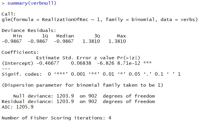
We see that the intercept is the logarith of the odds which we calculated above, and more importantly, the output for the null model in figure 10.4 shows identical null and residual deviances. This is the minimal model against which we are comparing our more expansive model which includes the verbs, the animacy of theme, and more importantly, the animacy of the recipient and the length of the theme. Observe that this intercept is the intercept of the null model and does not necessarily correspond to the intercept of the full model, the output of which we show in figure 10.3.

Of course, when we try to model the relationship between a dependent and several independent variables, we want our model to deviate from the data as little as possible. Intuitively, more information, i.e. more independent variables, enables for a more precise model. However, it is also possible to imagine cases where there is no relationship between the dependent and the independent variables in a model. In that case, including independent variables in the model would not decrease the residual deviance of the model compared to the null deviance. Accordingly, we compare the model we are interested in – the one with all the independent variables – to the bare-bones model – the one based solely on the odds of seeing a PP. This is where we return to the null and residual deviance in the summary output in figure 10.3.

If the null deviance is bigger than the residual deviance of the model, then the full model approximates the data better than the null model. This is the case in our example, where we have . By including the independent variables in our logistic regression model, we reduce the residual deviance by 634.86 while losing 67 degrees of freedom.^[1] This is how the null and residual deviance provide a first measure for the goodness of fit of our model.

Accuracy of prediction

https://uzh.mediaspace.cast.switch.ch/media/0_5xwy9ctn

In addition to comparing null and residual deviances, we can asses how good our logistic model is by using it to predict the dependent variable for each observation. Then we can compare the prediction with the observation and see how often the predictions match the observations. With a good model, the predictions will be equivalent to the observation very often.

In R, there is a function predict() which allows us to predict values based on our model. This function takes as its argument the model, verbfit, and the data. Here we want to work with the data on which the model is based, so we define data=verbs:

> verbs$predict = predict(verbfit, data=verbs)

If you look at the left-hand side of the equation in the command, you see that we are not assigning the predictions to a new variable. Instead, we add a further column called predict to the verbs data frame. It is to this new column that we save the predicted information. Since the model is constructed to explain the realization of the recipient using the information in the other columns, what we predict here is obviously the realization of the recipient.

Unfortunately, this is not at all obvious when we look at the output of the predictions:

> head(verbs$predict); tail(verbs$predict)
[1] -19.3688951  -1.4402943  -3.7333629  -2.2391271   0.1934832  -1.8901736
[1] -1.44029428 -1.44029428 -0.89046542  1.23626992 -1.89017364  0.05621641

This is clearly very different from the categorical output you might have expected. After all, we know that the observed data is always either NP or PP, never anything numeric. The numbers we see in the output here are actually the numerical output before we map them on the values 0 and 1, which then express the categories of NP and PP.

There is an option in the predict function which allows us to get more easily interpretable results, namely ‘type=response’. This gives us predicted values between 0 and 1, which means we can simply set a threshold at 0.5 to delimit the border between predicting one category, 0, or the other, 1:

> verbs$predictb = round(predict(verbfit, data=verbs, type="response"))

Notice that we simply overwrite the less interpretable output in the ‘predict’ column with these more meaningful predictions. If we look at the output now, we see a list of zeroes and ones:

> verbs$predictb

We see reflected here that all NP realizations are at the beginning of the table and all the PP realizations are at the end, so we see that zeroes correspond to NPs and ones correspond to PPs. This already gives us a little overview of the quality of the prediction: we see that in the beginning there are mostly zeroes and in the end there are mostly ones, but we also see that there are quite a few wrong predictions.

Now we want to compare the observed values to the values predicted by the model, and for this we can create a table which compares the realizations of the recipient and our predictions:

> confm = xtabs(~verbs$RealizationOfRec + verbs$predict)

We name this table confm for confusion matrix. This name can be taken literally, since it tells us how confused the model is, how often it confounds the categories and makes a wrong prediction. Let’s take a look it:

> confm
                      verbs$predictb
verbs$RealizationOfRec   0   1
                    NP 499  56
                    PP  69 279

We can see that in the top left cell, where we observe NPs and predict zeroes, we have 499, and in the bottom right cell, where we observe PPs and predict ones, we have 279. These are our correct predictions. Conversely, in the top right cell, where we observe NPs but predict ones, we have 56, and in the bottom left cell, where we observe PPs but predict ones, we have 69. These are our incorrect predictions. We can see that one diagonal, in this case top left to bottom right, contains the correct predictions and the other diagonal contains the wrong predictions.

A simple way to refer to these cells is by using the coordinates. This means we can add up the total number of correct predictions and divided it by the sum of predictions with the following command:

> (confm[1,1] + confm[2,2]) / sum(confm)
[1] 0.8615725

The calculation gives us the accuracy of prediction in percentage terms, so we can say that our model makes the correct prediction in 86% of the cases. This is a lot better than chance prediction, but the model is not extremely good. What is extremely good, however, is that we now have an interpretable measure for the quality of our logistic regression model. The accuracy of the prediction gives us a good indication for how reliable the trends we observe in the model summary are, and thus allows us to arrive at a better understanding of the data we are looking at.

In the previous chapter and the preceding example, we have discussed how regression analysis can inform linguistic research. In the next chapter, we present a very powerful implementation of the logistic regression model in LightSide, a machine learning tool for document classification.

Reference:

Kabacoff, Robert I. 2011. R in Action: Data Analysis and Graphics with R. Shelter Island, NY: Manning Publications.