In this chapter, we discuss the chi-square test. The affordance of the chi-square test is that it allows us to evaluate data of which we know that it is not normally distributed.
The chi-square test
https://uzh.mediaspace.cast.switch.ch/media/0_89u8aww7
In the last chapter, we introduced the t-test and saw that it relies crucially on the assumption that the data in our samples is normally distributed. Often, however, our data is not normally distributed. For these cases, we can use different significance tests that don’t assume a normal distribution.
Perhaps the most versatile of these is the chi-square test. In contrast to the t-test, which requires the mean, the standard deviation, the sample size and, of course, normally distributed data, the chi-square test works with the differences between a set of observed values (O) and expected values (E). The expected values either come from a model or from a reference speaker group. Frequently, you will calculate the expected values on the basis of the observed values, thereby generating your own model. We discuss how this works in detail below.
To calculate the chi-square value, expressed by the Greek letter  , the differences between observed and expected values are summed up. When we discussed the summation of differences in the context of the standard deviation, we saw that if we just sum the differences, positives and negatives cancel each other out. With the standard deviation, we work around this impasse by squaring the differences, and we can use the same approach to calculate the chi-square value. So, we square the difference between each observation and its corresponding expected value. Since we are not interested in the absolute differences, we normalize the squared differences before summing them, which gives us the following formula for the chi-square value:

As you can see, we normalize by E. We do this because the expected values are often more balanced than the observed values. This is already most of what we need for the chi-square test. Once we have the chi-square value, we can look up the probability of our results and see whether they are significantly different than what would expect if our data were just a bunch of random observations. That’s already the whole theory.
In the next sections, we discuss how the chi-square test is performed in practice.
Contingency tests
https://uzh.mediaspace.cast.switch.ch/media/0_7gndzy5q
A frequently used version of the Chi-square test is the contingency test, in which the expected values are the random distribution of the observed values. To illustrate what this means, let’s consider the following example which is based on Mukherjee (2009: 86ff). Here, we use data from the Lancaster-Oslo-Bergen (LOB) and the Freiburg-LOB (FLOB) corpora. The LOB contains texts from 1961 and the FLOB contains texts from 1991, and both corpora contain 500 texts of about 2,000 words each.
Let’s use the chi-square test to establish whether the usage of prevent NP from doing something (form 1) and prevent NP doing something (form 2) changed in British English between the 1960s and the 1990s. If we look at the table below, we see a clear difference: in the 1960s form 1 is predominant, while in the 1990s both forms are equally likely. But is this difference between the ’60s and ’90s statistically significant?
| form 1 | form 2 | row total | |
| LOB 1960s | 34 | 7 | 41 |
| FLOB 1990s | 24 | 24 | 48 |
| column total | 58 | 31 | 89 |
Before evaluting this, let’s formulate the hypotheses. The hypotheses for the chi-square test function similarly to those for the t-test, which means that we want to phrase a null hypothesis which we can reject in order to continue working with the alternative hypothesis. So, we can say:
HA: there is a difference in the usage of these forms over time.
Now, we could just enter our data into R and run a chi-square test on it, and we are going to do so below. But since working through this test manually enables a better understanding for how the test functions, we are going to do this first.
Performing the contingency test manually entails six steps:
- For every O calculate E
- Calculate the deviance of E from O
- Sum the values
- Calculate the degrees of freedom
- Decide on a significance level
- Check/calculate the critical values
Let’s walk through this step by step.
Step 1: For every O calculate E
The expected frequencies are “the frequencies that we would expect simply by chance (if the independent variable had no relationship to the distribution)” (Hatch and Farhady 1982: 166). Let’s look at an example before going into the LOB/FLOB data. If we look at foreign students enrolling for three different faculties at an American university, if there were 1,032 foreign students and three faculties (Sciences, Humanities, Arts) and the area of research were of no importance to students, we would expect that all faculties would get an equal number of foreign students, namely  . Our table would look like this:
| Sciences | Humanities | Arts | Row total | |
| Foreign students | 344 | 344 | 344 | 1032 |
However, because we have access to the enrollment data, we know how the numbers actually look. And the enrollment rates you observe look like this:
| Sciences | Humanities | Arts | Row total | |
| Foreign students | 543 | 437 | 52 | 1032 |
You can see that there is a substantial difference between our model, where all students are equally likely to enroll in any of the three faculties, and the observed data, which shows that some faculties clearly appeal to more students than others.
In our example with prevent NP, if the null hypothesis were true, we could assume that the two samples of British English from different periods are “a single sample from a single population” (Woods et al. 1986: 141). In other words, we assume that the number of occurrences for each of the two linguistic variants is independent of the time period. To calculate the expected values, then, we need the following formula:

For each cell, in row i and column j, we multiply the row total with the column total and divide the result by the grand total, which corresponds to the sum of all observations. Knowing this, you should be able to calculate the expected values for the observations in table 6.1. Write the expected values down in a table.
Step 2: Calculate the deviance of E from O
Remember that to calculate the  value, we will require the normalized differences:
  . Use this formula to calculate the normalized squared differences. Again, write them down in a table.
Step 3: Sum the values
This step gives us the chi-square value. We simply sum the normalized deviance of E from O:

Step 4: Calculate the degrees of freedom
We touched on the difficulty of degrees of freedom in the last chapter, but fret not: it is easy to calculate them for the contingency test. The number of degrees of freedom “is determined by the fact that if we know all but one value in a row or column, and also the row and column total, the remaining cell can be worked out. Therefore degrees of freedom = (no. of rows-1)*(no. of columns-1)” (Butler 1985: 121). In our example, this means: df = (2-1)*(2-1) = 1.
Step 5: Decide on a significance level
We have to do this whenever we perform a significance test. Let us stick with the conventions of linguistics and aim for significance level of 95%. This means that we want to have a probability of 95% that the difference between the two sets of data from the two time periods is not a matter of chance. In terms of the confidence value we discussed in the last chapter, we would want a p-value ≤ 0.05.
Step 6: Check the critical value

The table above contains the critical values for the value we calculated. How do we figure out the correct critical value? Well, we know that we have 1 degree of freedom, so we look at the first row, and since we decided on a 95% significance level, we look at the column under 0.05. Then we check whether the we calculated in step three is bigger than the critical value:

Since the calculated value is bigger than the critical value, we can reject the null hypothesis. In fact, the critical value at the 0.01 level is still smaller than our value, wherefore we can conclude that the difference between the two sets of data is highly significant at the 1% level. In other words, there is a likelihood of 99% that the difference we observed in the usage of the two forms is not a matter of chance. This means that we can reject the H0 and assume that HA is true: there is a difference in the usage of the two forms over time.
The reasoning behind this conclusion becomes clear when we look at how the chi-square value is defined:
The corresponds to the total deviation of the observed and the expected values, and the difference between the two is too high for the H0 to be true.
Exercise: contingency test in Excel
https://uzh.mediaspace.cast.switch.ch/media/0_goqkfp5b
Before moving to a higher abstraction, which is the chi-square test in R, try solving the contingency test in Excel. Use the formula discussed above to calculate the expected values, and then us the Excel function CHISQ.TEST(). Copy the table below into Excel to get started. In the video above, Gerold walks you through the steps, but we recommend you try it yourself first before checking out the solution in the slides below:
As you can see, Excel automates one step for you: you no longer have to look up the critical value. Instead, the output of the Excel function is the probability of H0 being true. This means that you come to conclusion we had above simply by interpreting the Excel output correctly.
Chi-square distribution
In Introductio to Inferential Statistics we saw how the normal distribution naturally arises. You probably were not really surprised when you saw the bell shape of the normal distribution. Like the normal distribution, the chi-square distribution arises naturally, but its shape is far from intuitive.
We’ll show you what we mean by this while we discuss how to generate a chi-square distributions in R. First, we define four normally distributed variables, each with mean of 0, a standard deviation of 2 and 10,000 observations:
> x=rnorm(10000,0,2)
> y=rnorm(10000,0,2)
> z=rnorm(10000,0,2)
> w=rnorm(10000,0,2)
If you visualize any one of these four variables as a histogram, you will just see a normal distribution:
> hist(x, breaks=100, freq=F)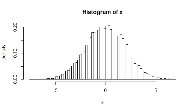
This changes drastically if you square x and plot it again:
> x2=x^2
> hist(x2, breaks=100, freq=F)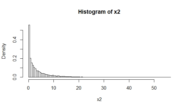
We use the variables from above to generate sums of independent, squared and normally distributed random variables:
> xy2 = (x^2+y^2) # sum of 2 squared normal distributions
> xyz2 = (x^2+y^2+z^2) # sum of 3 squared normal distributions
> xyzw2 = (x^2+y^2+z^2+w^2)    # sum of 4 squared normal distributions
Now we can use these sums to plot the different chi-square distributions with different degrees of freedom:
> hist(x2,breaks=100,xlim=c(0,40),ylim=c(0,0.2),freq=F)
> hist(xy2,breaks=100,add=T,freq=F,col="#0000ff66") # df = 2
> hist(xyz2,breaks=100,add=T,freq=F,col="#ff000066") # df = 3
> hist(xyzw2,breaks=100,add=T,freq=F,col="#00ff0066") # df = 4
You can see that the chi-distribution changes drastically with each change in the degrees of freedom. This is why it is essential to know how many degrees of freedom we have when running a chi-square test.
As with the t-distribution, we require the chi-square distribution to derive the critival value. In the example above, we calculated  with df=1. Now, we visualized a chi-square distribution with 1 degree of freedom and saw that most of the values are very close to one. In fact, we looked up the critical value for the 0.05 significance level which told us that 95% of all values in a chi-square distribution are smaller than 3.84. So, the chi-square distribution functions as a benchmark for our expectations, just as the t-distribution does for the t-test.
Chi-square test in R
https://uzh.mediaspace.cast.switch.ch/media/0_ug7lwwdv
A note on the video: the links to the web calculators Gerold refers to are located at the end of the chapter.
We mentioned earlier that using R for a chi-square test is more abstract from the contingency test than using Excel is. The simple reason for that is that R does not require us to calculate the expected values. This is best illustrated with an example.
Let’s replicate the prevent NP (from) doing data in R. We can do this by creating two vectors which contain the data. Assign the data from the 1960s to the variable lob and the data from the 1990s to the variable flob:
> lob=c(34,7) ; flob=c(24,24)In the next step, we need to create a table from these two vectors. We can do this by assigning the output of the data.frame() command to a new variable:
> lobflobtable <- data.frame(lob,flob)data.frame() takes the data variables as arguments and forms a table from them.
Now, we can simply use the inbuilt chisq.test() function on our table which contains the observed values. The expected values are calculated automatically and are not displayed. When you enter the chisq.test command, the output looks like this:
> chisq.test(lobflobtable)

	Pearson's Chi-squared test with Yates' continuity correction

data:  lobflobtable
X-squared = 9.1607, df = 1, p-value = 0.002473
You can see that R calculates value and the degrees of freedom and gives us the p-value. With a p-value = 0.002473, the R output looks slightly different than our Excel results above. The reason for this is that R automatically includes the so-called Yates’ continuity correction, which aims at alleviating an error introduced by the assumption that the discrete probabilities of frequencies can be approximated by a continuous distribution.
Pitfalls of chi-square: conditions of usage
As with every other significance test, the chi-square test has very clear conditions of usage that we have to consider in order to attain reliable results. There are three general conditions which should be considered when working with the chi-square test.
The first of these is that absolute frequencies have to be used for the chi-square test. If you convert absolute frequencies into relative or normalized frequencies, the chi-square value may appear highly significant when in fact it wouldn’t be with absolute frequencies (Woods et al. 1986: 151). Thus, performing a chi-square test with normalized or relative frequencies is misleading, and should not be done.
The second important condition is that all observations have to be independent from each other (Gries 2008: 157). Woods et al. state that “whenever it is not clear that the observations are completely independent, if a chi-square value is calculated, it should be treated very skeptically and attention drawn to possible defects in the sampling method” (1986: 149).
The third condition is that “each observation must fall in one (and only one) category” (Hatch and Farhady 1982: 170). In other words, the categories have to be mutually exclusive.
Two further features of the chi-square test are concerned with specific cases. The first of these is the Yates’ correction, which has to be applied “for one-way and 2×2 tables where the df is only 1” (Hatch and Farhady 1982: 170). The Yates correction factor is defined as follows: “0.5 is added to each value of O if it is less than E, and 0.5 is subtracted from each value of O it is more than E” (Oakes 1998: 25). Thus, the Yates’ correction is applied in cases with a minimum degree of freedom. The second is that the chi-square test does not work with low expected frequencies. The frequencies are too low to work with when at least one of the expected frequencies lies below 5 (Mukherjee 2009: 88). In other words, if we have very few observations or very few dimensions in the data, the chi-square test works less reliably than if we have more of either.
Then, of course, there is a more general problem with very high frequencies and the assumption of random generation of natural language: “For all but purely random populations,  tends to increase with frequency. However, in natural language, words are not selected at random, and hence corpora are not randomly generated. If we increase the sample size, we ultimately reach the point where all null hypotheses would be rejected” (Oakes 1998: 28f, also see Mukherjee 2009: 89). This does not prevent linguists from using the chi-square test, and it does not generally invalidate the use of the chi-square test. But knowing this, you might want to consider using a different test if the chi-square test identifies things that look very similar as being different.[1]
Finally, you should be aware of what the chi-square test can and cannot be used for. The chi-square test “does not allow to make cause and effect claims” (Oakes 1998: 24). It will only “allow an estimation of whether the frequencies in a table differ significantly from each other” (Oakes 1998: 24). Thus, while the chi-square test is very useful to identify whether the patterns we observe in the data are random or not, it falls short of actually allowing us to make causal claims. In order to make those, we need some more advanced statistical methods like the regression analysis which we discuss in Advanced Methods.
Useful web links
Before we progress to the next chapter, we should point out that there are several online calculators which run the chi-square test for you. At the time of writing, these include:
- http://statpages.org/#CrossTabs
- http://www.physics.csbsju.edu/stats/contingency_NROW_NCOLUMN_form.html
- http://www.mirrorservice.org/sites/home.ubalt.edu/ntsbarsh/Business-stat/otherapplets/Catego.htm
Due to the nature of the web, links change very often, and we cannot guarantee that these links will work. If they do, however, they are a useful resource if you want to run a quick chi-square test without access to Excel or R.
References:
Butler, Christopher. 1985. Statistics in Linguistics. Oxford: Blackwell.
Gries, Stefan Th. 2008. Statistik für Sprachwissenschaftler. Göttingen: Vandenhoeck & Ruprecht.
Hatch, Evelyn Marcussen, and Hossein Farhady. 1982. Research design and statistics for applied linguistics. Rowley, Mass: Newbury House.
The LOB Corpus, original version. 1970–1978. Compiled by Geoffrey Leech, Lancaster University, Stig Johansson, University of Oslo (project leaders), and Knut Hofland, University of Bergen (head of computing).
Mukherjee, Joybrato. 2009. Anglistische Korpuslinguistik – Eine Einführung. Grundlagen der Anglistik und Amerikanistik 33. Berlin: Schmidt.
Oakes, Michael P. 1998. Statistics for Corpus Linguistics Edinburgh. Edinburgh: EUP.
Woods, Anthony, Paul Fletcher and Arthur Hughes. 1986. Statistics in Language Studies. Cambridge: CUP.
- See, for instance, the 'chi by degrees of freedom' in Oakes 1998: 29 ↵
