In this first part of the book, the Foundations, we want to make sure that everyone has a practical understanding of the programming language R, which we use throughout. In this chapter, you will make your first steps in R and learn how to import data into the program.

 

What is R?

https://uzh.mediaspace.cast.switch.ch/media/0_deh5auqn

The R project page is http://www.r-project.org/. Download the program for your OS from the ETH mirror http://stat.ethz.ch/CRAN/. Install as you usually install programs. Once you have installed the R base, you have all the tools you need for the next chapters at your disposal.

Nonetheless, you might want to consider installing RStudio on top of the R base. RStudio is an integrated development environment which allows you to keep track of the data and variables you are using. Moreover, when you are writing a piece of code composed of several commands, the script window in RStudio allows you to break it down into one command per line. If you think these functionalities sound helpful, download RStudio Desktop from https://rstudio.com/products/rstudio/ and install.

R base and RStudio have somewhat different graphic user interfaces, as you can see below. In R base, there is only one window: the console. The console is where you communicate with the program. Here, you enter the commands you want R to execute, and it is where you see the output. In most programming languages, including R, you can recognize the console by the prompt, which looks like this: >.

In RStudio, there are four windows. The top left window is the script. Here you can enter multiple lines of code without immediately executing them. The top right window shows the global environment. Here you find all the data and variables in use in your current session. The bottom left window is where plots will be displayed. Finally, and most importantly for now, you find the console in the bottom left window. This corresponds to the R base console in that the commands you enter here will be executed immediately.

In the video tutorials, you see Gerold working with R base. If you are using RStudio, you will want to try what Gerold does in the console.

https://uzh.mediaspace.cast.switch.ch/media/0_quelm2x2

When you start R, the prompt > appears in the console. Select the console window, and type your first command:

> 2+2

When you hit enter, R executes your command and gives you the output. The output here is:

[1] 4

You are hopefully not surprised. You have just used R as a calculator, and this if a very legitimate way to use it. However, the program is capable of doing much more, and we begin exploring the possibilities in this chapter.

Let us begin by importing some data, such as the file verbs.txt.^[1] Take a look at this raw text file by opening it in a new browser tab:

verbs.txt

You may have the impression that the table looks skewed, that not all rows are aligned. This is no reason to worry: it is simply because the fields are separated by tabulator characters. Tabulator-separated fields are very flexible, a simple de facto standard which allows us to import data into spreadsheets like Excel or databases like FileMaker.

To save the file on your computer, right-click on the link and select “Save As…”. The image below shows this step in a German version of Firefox:

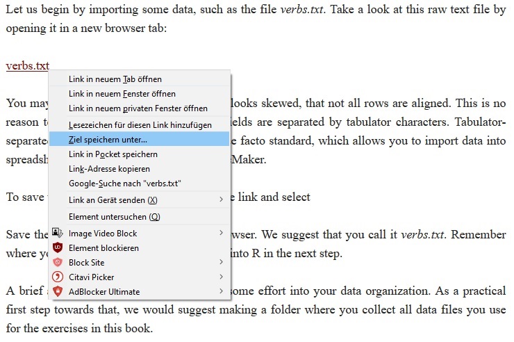
Save the file as a raw text file from the browser. We suggest calling it verbs.txt. Remember where you save it, because you will need to know the file’s location in order to import it into R in the next step.

But first, a brief comment on saving files: it is generally worth putting some effort into organizing your data and folder structure. As a practical step towards that, we would suggest creating a folder where you store all data files that you download over the course of the book. Of course, you can create subfolders according to chapters, or topics, or whatnot, depending on your personal preferences. But being somewhat inundated with files ourselves, we cannot overstate the value of having a system for data storage.

Returning to R, you can load the verb.txt file via the console. When you enter the following command, a dialogue window will open:

> verbs <- read.table(file.choose(), header=TRUE, comment.char="", row.names=1)

In the dialogue window, navigate to the folder where you stored the file, and open the verbs.txt text file. When you open verbs.txt, you assign it to the variable verbs. This what the arrow construction, <-, effects. The variable verbs now contains the table that you opened in the browser earlier.

 

What is a variable?

In this section, we loosely follow chapter 1 in Baayen (2008).

https://uzh.mediaspace.cast.switch.ch/media/0_v7pi1adx

What are we talking about when we say that you assigned the table verbs.txt to a variable verbs? We are not talking about linguistic variables (not just yet), but about computational variables. In R, variables are objects to which you can assign different values. At its simplest, a variable contains a single value. Consider the following example:

> x <- 1 + 2
> 1 + 2 -> x
> x
[1] 3

In this example, we assign the outcome of a simple calculation to the variable x. And when we tell R to show x, the output is the outcome of the calculation.

With this in mind, consider again what we did with the verbs variable. We assigned a whole table to it, and we can look at it. However, since the whole table is too big to be represented usefully in the R console, let’s just take a look at the first few rows. We can do this with the head() command:

> head(verbs)
  RealizationOfRec  Verb AnimacyOfRec AnimacyOfTheme LengthOfTheme
1               NP  feed      animate      inanimate      2.639057
2               NP  give      animate      inanimate      1.098612
3               NP  give      animate      inanimate      2.564949
4               NP  give      animate      inanimate      1.609438
5               NP offer      animate      inanimate      1.098612
6               NP  give      animate      inanimate      1.386294

By default, head() shows the first six rows. To view the first 10 rows, we can modify head() with the argument n=10:

> head(verbs, n=10)
   RealizationOfRec  Verb AnimacyOfRec AnimacyOfTheme LengthOfTheme
1                NP  feed      animate      inanimate     2.6390573
2                NP  give      animate      inanimate     1.0986123
3                NP  give      animate      inanimate     2.5649494
4                NP  give      animate      inanimate     1.6094379
5                NP offer      animate      inanimate     1.0986123
6                NP  give      animate      inanimate     1.3862944
7                NP   pay      animate      inanimate     1.3862944
8                NP bring      animate      inanimate     0.0000000
9                NP teach      animate      inanimate     2.3978953
10               NP  give      animate      inanimate     0.6931472

Now that we have imported the data into R and taken a first look at it, one question remains unanswered: what does it mean?

 

How is the data to be interpreted?

https://uzh.mediaspace.cast.switch.ch/media/0_9vhnuvjp

The table verbs contains linguistic data on the realization of ditransitive verbs. Each row represents one instance of a ditransitive verb from a corpus. The columns contain information on several aspects of each realization:

• RealizationOfRec: is the recipient an NP (as in I gave you a book) or a PP (as in I gave a book to you)?
• Verb: which ditransitive verb is used in this instance?
• AnimacyOfRec: is the recipient animate?
• AnimacyOfTheme: is the theme animate?
• LengthOfTheme: how long is the theme?

We can see immediately that there are different types of scale in this data. Three of the columns, RealizationOfRec, AnimacyOfRec and AnimacyOfTheme contain nominal variables. This means that they can take one of two mutually exclusive values. A recipient can be realized either as an NP or a PP, but it cannot be anything in between or any thir option. The same is evidently true of the animacy of the recipient and theme. English does not have a third mode of animacy for the half-dead. The Verb column contains what is known as a categorical variable. Again, we have mutually exclusive categories, but this time we have more than two categories. What nominal and categorical variables have in common is that even if we translate the categories into numbers – which can be very useful – the number we assign a value does not weigh in a mathematical way. In other words, even if the categories are described numerically, we do not rank them the way we would rank numerical data. In the final column, LengthOfTheme, we actually do have numerical data. As we can see from the first few lines, the length of the theme is a continuous numeric variable. This table then contains the most important types of scales we use in linguistics.

Which brings us back to the question: how can we interpret a table like this linguistically? Well, this dataset can, for example, be used to find out if certain verbs have a preference for realizing the recipient as a noun phrase (NP) or a prepositional phrase (PP). But before we dig deeper into how we can evaluate data like this with statistical methods, which we will do in later chapters, let’s look in some more detail at our variable verbs as an object in R.

As you know, verbs is a table. In R, tables are referred to as data frames. In this book, we talk about both tables and data frames, in both cases to referring to structured data arranged by rows and columns. The differences is that we use tables generally, and data frames only when we talk about the objects in R.

When we are handling a data frame in R, it is possible to view specific values:

> verbs[1,]   # displays row 1
> verbs[,1]   # displays column 1

When displaying an entire row, the output shows the value in each column of that row. When displaying an entire column, the output shows the value in each row of that column.

If you use the square brackets to take a look at each of the five columns, you will see that the output of the first four columns conatins an additional line after the contents of the 903 rows. This line is titled Levels, and it contains a list of the categories in these columns. In other words, the levels are the different values nominal and categorical data takes. In this line we see that the RealizationOfRec can be either a “NP” or a “PP”, and we see that there are 65 verbs, from “accord” to “wish”.

We can also view the levels with the command levels():

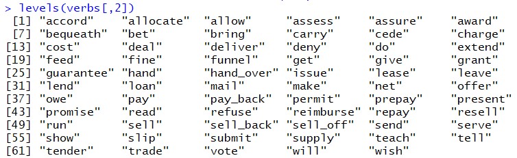
Here you see, for instance, all of the 65 verbs. Looking at levels like this comes in especially handy if you are not certain what your dataset contains in detail, for instance when you download something in the context of a textbook, and want to see whether it features that one verb you are interested in.

If you look at the last column, you will see that R does not give you a Levels line in the output. This is because numerical data can theoretically take an infinte number of values and accordingly is not structured in levels the way categorical data is.

Continuing the work with the square bracket queries, we can look up the value of an specific cell. For instance, we can look at row 401 in the AnimacyOfRec column using the following command:

> verbs[401,3]
[1] animate
Levels: animate inanimate

We can also formulate more complex queries and search, for instance, using ranges. In R, we express ranges with a colon, as in 2:5. Consider the following search query:

> verbs[2:5,1:3]
  RealizationOfRec  Verb AnimacyOfRec
2               NP  give      animate
3               NP  give      animate
4               NP  give      animate
5               NP offer      animate

You see that with these range searches, R displays rows 2 through 5 and columns 1 through 3.

Alternatively, we can restrict our searches to small selections. We do this by using the command c(). This command combines values into a vector or list. You could also think of c() as a command to concatenate.

Say we want to look at rows 1 to 6, but for some reason we really don’t want the third row to be displayed. We can do this using c():

> verbs[c(1,2,4,5,6),]

We can, of course, do the same thing for columns:

> verbs[,c(1,3)]

All of the search queries we looked at so far are concerned with how to access certain positions in a data frame. But usually we are less interested in seeing a specific cell than looking at certain values.

 

How can we formulate queries for specific values?

https://uzh.mediaspace.cast.switch.ch/media/0_7qvq0p4y

When the contents of a cell (or several cells) interest us more than its position, we can formulate something like a database query. For instance, we may be interested in seeing all rows in verbs which have an animate theme. In this case we would type the following command:

> verbs[verbs$AnimacyOfTheme == "animate",]
    RealizationOfRec  Verb AnimacyOfRec AnimacyOfTheme LengthOfTheme
58                NP  give      animate        animate     1.0986123
100               NP  give      animate        animate     2.8903718
143               NP  give    inanimate        animate     2.6390573
390               NP  lend      animate        animate     0.6931472
506               NP  give      animate        animate     1.9459101
736               PP trade      animate        animate     1.6094379

This query looks more complex than anything we have seen so far, so let’s break it down. As before, we have verbs followed by square brackets. This means that we want to access the content of the variable verbs as defined by the criterion in the square brackets. In the square brackets we have verbs$AnimacyOfTheme which means that within verbs, we want only those cases in which the animacy of theme is animate. The two equal signs are used to test for exact equality, and this is what gives us the desired output.^[2] This type of query takes some getting used to, but it is how R allows us to do something like a database query.

With this understanding, you can easily formulate analogous queries for different criteria:

> verbs[verbs$Verb == "lend",]

Of course, these can be expanded to include multiple elements:

> verbs[verbs$Verb=="lend" | verbs$Verb=="sell",]

The | means “or”, so R displays all the rows containing either the verb “sell” or “lend”.

Now, our data frame has multiple columns of categorical data, so we can use this syntax to search for rows which are consistent with two conditions:

> verbs[verbs$Verb=="lend" & verbs$RealizationOfRec=="PP",]

As you would expect the & means “and”, wherefore the output contains those rows in which the recipient of the word lend is realized as PP.

That’s it! You have seen how to import data and phrase search queries, and you will learn more about R in the next chapter, Introduction to R.

 

Reference:

Baayen, R. H. (2008) Analyzing Linguistic Data. A Practical Introduction to Statistics Using R. Cambridge University Press, Cambridge.

---