In this chapter we discuss document classification, a common application of logistic regressions, and present an example using the software LightSide.

Introduction to document classification

https://uzh.mediaspace.cast.switch.ch/media/0_vvgu8uz2

Although it would be possible to perform document classifications in R, we decided to use a free, sophisticated and user-friendly tool specifically designed for document classification: LightSide. Since we do not have a dataset which we can make available for you directly, you will not be able to replicate the example we present here. Still, we can only encourage you to download LightSide here, install it using their excellent user manual (Mayfield et al. 2014) and play around with some data that interests you.^[1] In the unlikely event that you should find LightSide too daunting to dive into it head first, it should still be possible to follow the discussion below without performing each step along the way yourself.

Before we get into the details, however, we should say a few words about document classification. Document classification is an important branch of computational linguistics since it provides a productive way handle large quantities of text. Think for a moment about spam mails. According to analysis of the anti-virus company Kaspersky, more than half of the global email traffic is spam mail (Vergelis et al. 2019). How do email providers manage to sift these quantities of data? They use document classification to separate the important email traffic from spam mail. And how does document classification work? Essentially by solving a logistic regression.

When we discussed the logistic regression in the preceding chapter, we chose a set of explanatory variables to predict the outcome of categorical dependent variable. Since LightSide is a machine learning-based application, we don’t have to define the explanatory variables beforehand. Instead we let LightSide select the features. In fact, LightSide uses all of the features in the documents we want to classify and it automatically identifies which words are most indicative of each class.

To begin with, we need to open LightSide. If you installed it following the manual’s description, you should be able to launch it on a Windows computer by opening the ‘LightSIDE.bat’ file in the ‘lightside’ folder. On a Mac, you should be able to run LightSide by downloading the zip folder from the webpage, unzipping it, selecting ‘lightside.command’ with a right-click, choosing ‘open with’ and then selecting ‘terminal’. A window will pop open asking you whether you are sure you want to open this file, and there you can select yes. Now, LightSide should launch.

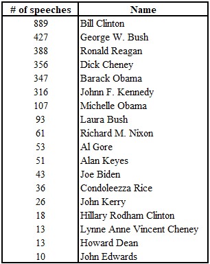
Once LightSide is open, the first thing we need to do is select the corpus that we want to classify. In our example, we work with Guerini et al.’s (2013)  CORPS 2 which contains more than 8 million words from 3618 speeches. Most of the speeches are by American politicians, but the corpus also includes speeches by Margaret Thatcher. The question we are asking is whether we can determine a politician’s party only on the basis of their speeches. We are going to use speeches by those politicians who are either Democrat or Republican and who are represented by more than 10 speeches. Since the corpus is from 2013, the most recent developments in American politics are, of course, not captured here.

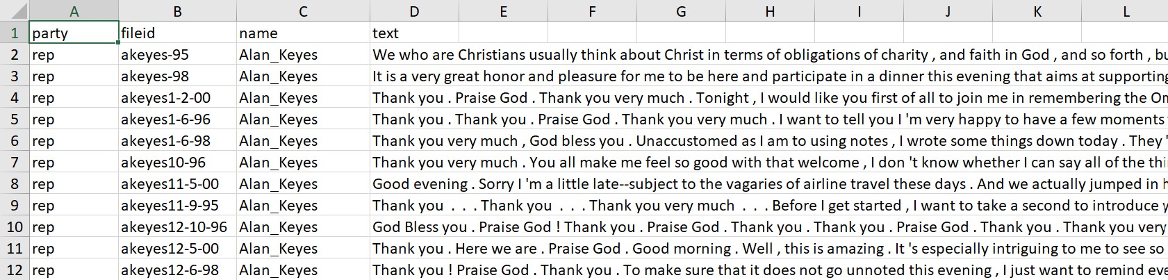
We had to pre-process the speeches with some simple steps, and we want to show you the final form of the data so that you can get an idea of what the input for LightSide should look like. In the screenshot below, you see how the comma separated data looks in Excel. In the first column, we have the party affiliation which is either ‘rep’ or ‘dem’. The second column shows the file id. The third column contains the politician’s name. As you might guess from only seeing Alan Keyes in the first rows, the table is sorted alphabetically according to the politician’s name. Each cell in the fourth column contains an entire speech.

Importing data into LightSide

https://uzh.mediaspace.cast.switch.ch/media/0_d0zin257

When we load this table into LightSide, each of the words in the speeches is converted into an appropriate representation. For the documents it uses a vector space model, which we do not explain in detail since it is beyond the scope of this introduction. At this stage it suffices to know that each word is going to be turned into a feature, on the basis of which LightSide will make its predictions of the politicians’ party. The fact that some words are more typical of one party can be leveraged to predict which party a given speech belongs to. Since we have 18,175 types, we have very many features which LightSide can use to construct a model.

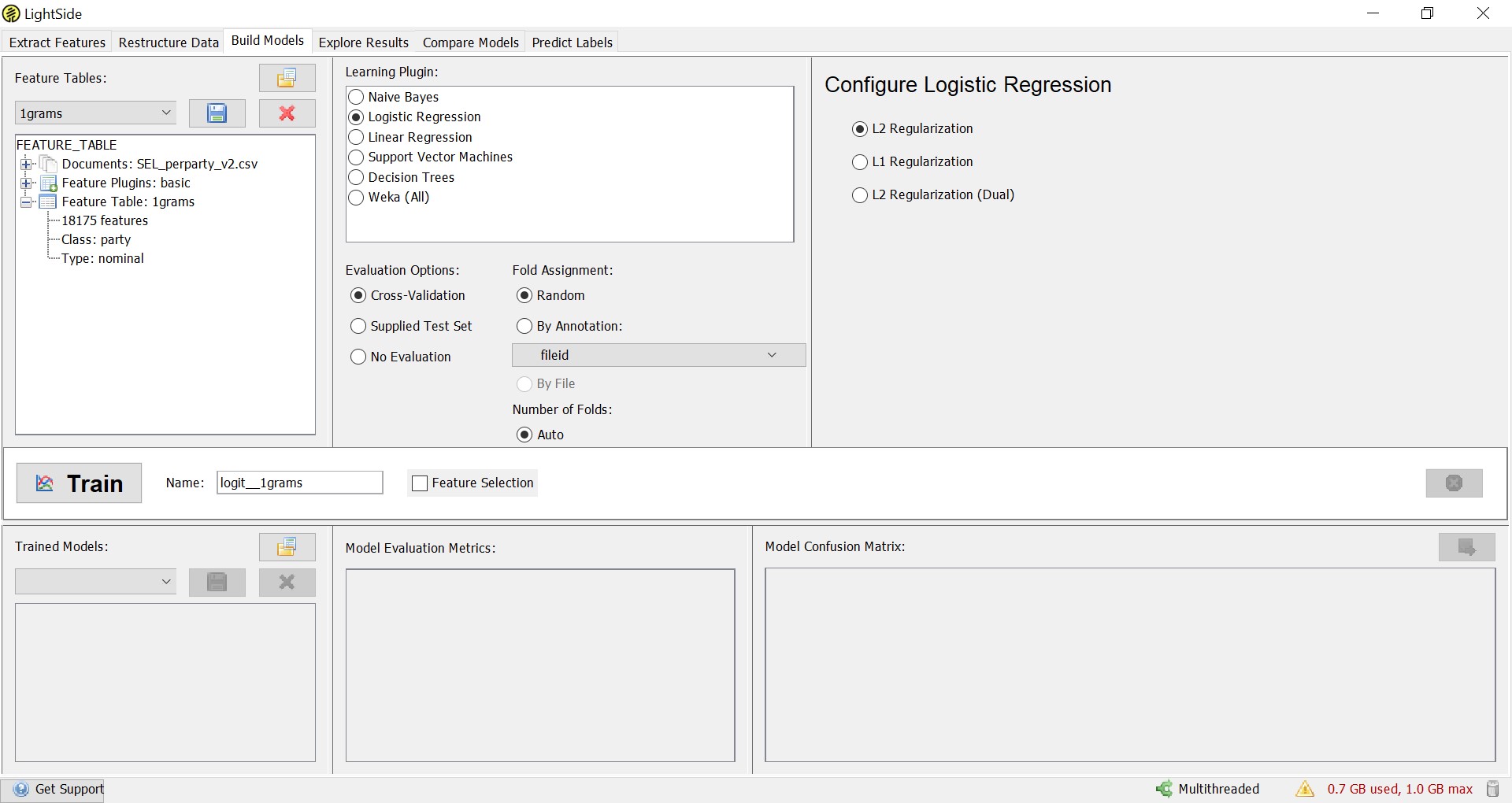
As figure 11.1 shows, the LightSide window is divided into an upper and a lower half. Each of these halves is divided into three columns. First, we work through the columns in the upper half from left to right. To import a .csv file into LightSide, click on the little folder icon in the upper left column. A window will open, and you can drag-and-drop the file containing your text collection into this window. Once the corpus is imported, select the ‘Class’ to tell LightSide what you want to predict. In our example, we use the class ‘party’ since we are interested in identifying party affiliations. The party is a binary, nominal type of class, just like the realization of the recipient was in the last chapter on the logistic regression. LightSide automatically identifies party as such a binary class. We want to predict the party from the information in the ‘text’ column in our data, so we select that in the ‘Text Fields’ tab.

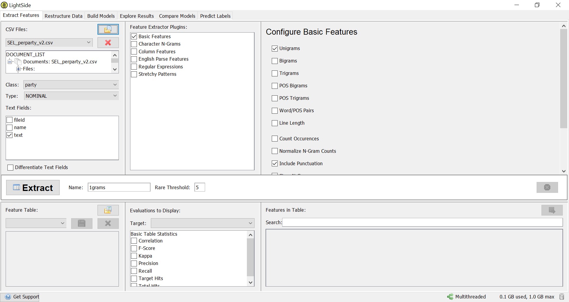
After setting these parameters, we can choose in the middle and right column which types of features we want LightSide to use for the prediction. In our example, we only use ‘Unigrams’ from the ‘Basic Features’.^[2] Accordingly, we want to know which individual words are indicative of party affiliation. This is also known as a bag-of-words approach, since we do not regard word combinations at all here. When using LightSide for research purposes, it makes sense to play around with and compare different models based on different features.

Once we have selected the features we want LightSide to use, we can extract them by clicking on the ‘Extract’ tile. On the same height as the ‘Extract’ button but on the right side of the LightSide window, there is a counter telling us how many features have already been extracted. Depending on the corpus size, this may take a while.

Building a model with 1-gram features

https://uzh.mediaspace.cast.switch.ch/media/0_p5l0a0sg

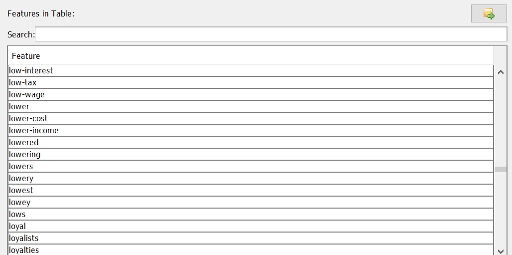
Once the features are extracted, we turn to the lower half of the screen. In the lower left column, the most interesting thing to note is the information of how many features are in our feature table. In our example, we have 18,175 features. The lower middle column gives us the option of looking at different metrics for each feature. While this can be useful at more advanced levels, we can ignore this at the moment. In the bottom right panel, we see our feature table in alphabetical order. In our example, this begins with a lot of year numbers, but if we scroll through the table, we see that the overwhelming majority of the features are words. Table 11.3 is a screenshot taken somewhere in the middle of our feature table.

With the extracted features, we can jump directly to creating a model. To do so, we have to go to the ‘Build Model’ tab. Here we can select which algorithm we want our model to be based on. Of course, in our example we choose ‘Logistic Regression’, since this is the type of model which interests us here. What changes now in comparison to the example in the last chapter is that instead of a few dozen, we now use thousands of features to predict the dependent variable. The capability of handling very large numbers of features is one of the great affordances of machine learning.

Another important difference between this implementation of the logistic regression and the generalized linear model we saw in the last chapter is the ‘Cross-Validation’, which we can select in the ‘Evaluation Options’. This means instead of training the model on all of the available data, we train it on 90% of the data and then apply it to the remaining 10% of the data. This is done ten times, and each time a different 10% is excluded from the training data. This is known as 10-fold cross-validation, and it means that actually ten different models are being trained on ten different selections of the data. Then, the mean of the parameters of these ten models is taken to construct the final model. We can create the model by clicking the ‘Train’ tile. Again, this may take a while, and we can follow the progress with the counter, where we see which of our ten  folds are testing.

Evaluating the model

https://uzh.mediaspace.cast.switch.ch/media/0_g278bvaq

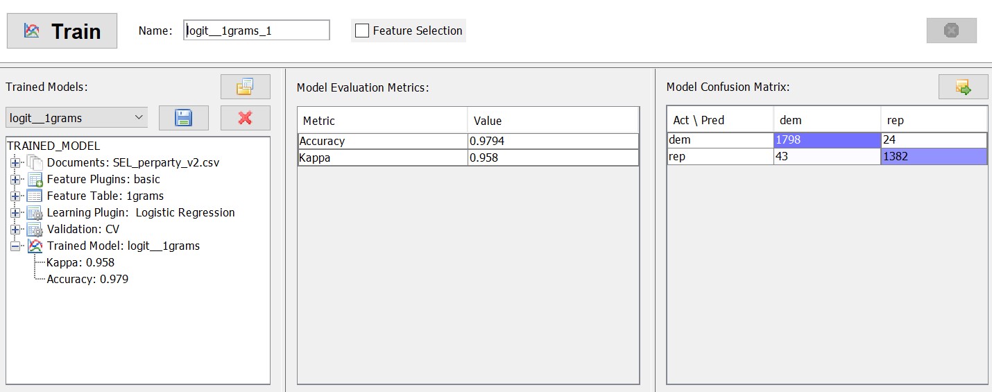
The results are presented in the lower half of the window. In the lower middle column, we see the accuracy of the model. In our example, we get an accuracy of 97.9%, meaning that only about 2% of the speeches were classified incorrectly. The Kappa value expresses how much better our model is than the random choice baseline. The value of 0.957 we see here means that our model performs 95% better than if we classified the speeches at random. This is very similar to the null-model against which we compared our logistic model in the last chapter. In the lower right column, we see the actual confusion matrix, which tells us how many speeches were predicted correctly. All of these measures indicate that we can predict a politician’s party quite reliably solely on the basis of the words in the speech.

For our linguistic purposes, it’s very interesting to look at the feature weight, which is a measure for the importance of each feature for the model. To do this, we can go to the ‘Explore Results’ tab. Let’s say we are interested in seeing the most typical Republican features. We can do this by ticking the box in the confusion matrix where the predicted and actual Republican outcomes intersect. Then we can choose the ‘Frequency’ and the ‘Feature Influence’ among the ‘Evaluations to Display’.

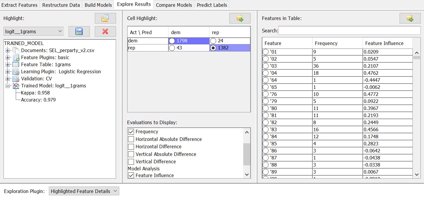
Now, we can sort the feature table in the upper right column according to the feature weight by clicking on the ‘Feature Influence’ tile. The negative features are strongly indicative of the Democratic party, while the positive features are strongly indicative of the Republican party.^[3] The closer the feature influence is to zero, the less explanatory power it holds. Let’s take a look at the features most indicative of being Republican:

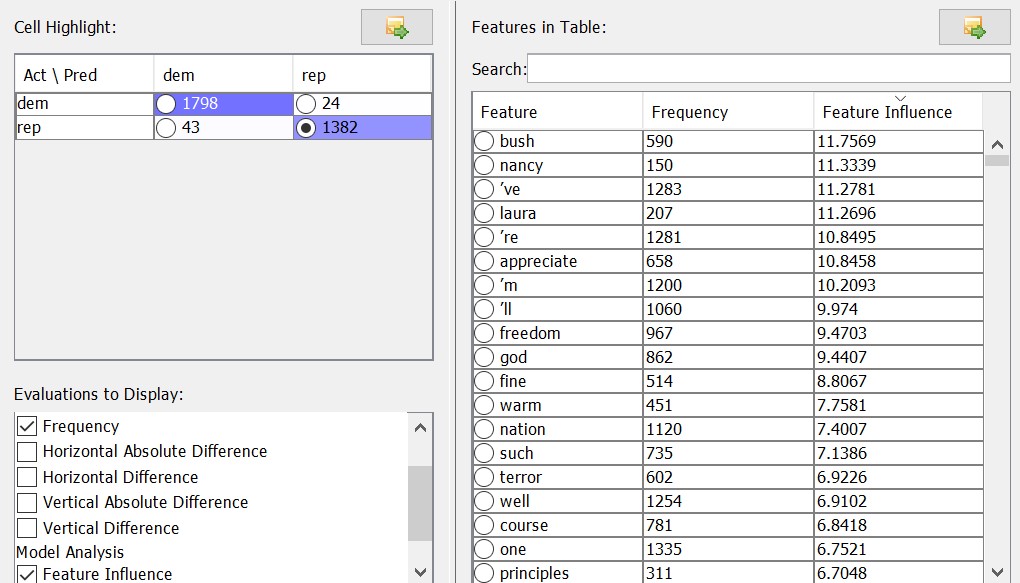
We see among the most Republican features several names – Bush, Nancy (Reagan), Laura (Bush) – and several familiar buzzwords – freedom, god, nation, terror. Linguistically, it is interesting to note that contractions – ‘ve, ‘m, ‘ll – are decisively Republican features. A first interpretation of this could be that Republicans want to present themselves as being close to the public, using colloquial language rather than technical jargon.

Of course, if one were to pursue this line of investigation seriously, one would have to check whether these results are the consequence of different transcription conventions, and whether there is evidence of the ‘one of the people’ attitude in the speeches of Republicans (and how Democrat politicians present themselves). We are not going to expound on this at any greater length, but this example should demonstrate both how unigram features can provide a good basis for further analysis and how these features should be interpreted with some caution.

We see here how regression analysis provides a basis for understanding advanced machine learning tools such as LightSide. What we also see is how we strain the limit of interpretability when we perform regression analysis on this scale: in our example we have about 18,000 features which contribute to the model, which is in excess of what can be incorporated in a qualitative analysis. This problem is not limited to document classification. Whenever we want to analyze substantial quantities of text, human reading capacities are challenged. We are going to discuss topic modelling in the next chapter to address this issue of excess information.

References:

Guerini M., Giampiccolo D., Moretti G., Sprugnoli R., & Strapparava C. 2013. The New Release of CORPS: A Corpus of Political Speeches Annotated with Audience Reactions. Multimodal Communication in Political Speech: Shaping Minds and Social Action, ed. by Isabella Poggi, Francesca D’Errico, Laura Vincze and Alessandro Vinciarelli, 86-98. Berlin: Springer.

Lightside

Mayfield, Elijah, David Adamson and Carolyn P. Rosé. 2014. LightSide: Researcher’s Workbench User Manual. Online: http://ankara.lti.cs.cmu.edu/side/LightSide_Researchers_Manual.pdf.

Vergelis, Maria, Tatyana Shcherbakova and Tatyana Sidorina. 2019. Spam and phishing in Q1 2019. Kaspersky. Online: https://securelist.com/spam-and-phishing-in-q1-2019/90795/.