In this chapter, we will take a step back and discuss several defining features of R. If you are not yet familiar with any programming language, you will learn the conventional terminology and get to know practical and common concepts of programming.

 

Why R?

https://uzh.mediaspace.cast.switch.ch/media/0_2zy3cc4p

In the last chapter, we saw how R can be used to get a handle on large data sets, and if you got this far, there will be no need to recapitulate how statistics can augment linguistic research. If, however, you already know another programming language you might wonder why you should learn R. Well, there are several reasons:

• It’s very close to statistics
• It’s powerful, as you will see later on
• It makes minimal use of procedural style and has a functional flavor
• There are many libraries for specific tasks
• The code is often less hackish than e.g. Perl
• It has less syntactic overhead than e.g. Perl
• It is less verbose than e.g. Java
• It is conceptually easier than Prolog

And, of course, different languages are useful for different purposes. Don’t use R instead of, but in addition to the languages you already know. There are, for example, APIs from Perl, Prolog and Python to R which allow you to integrate the different languages with each other.

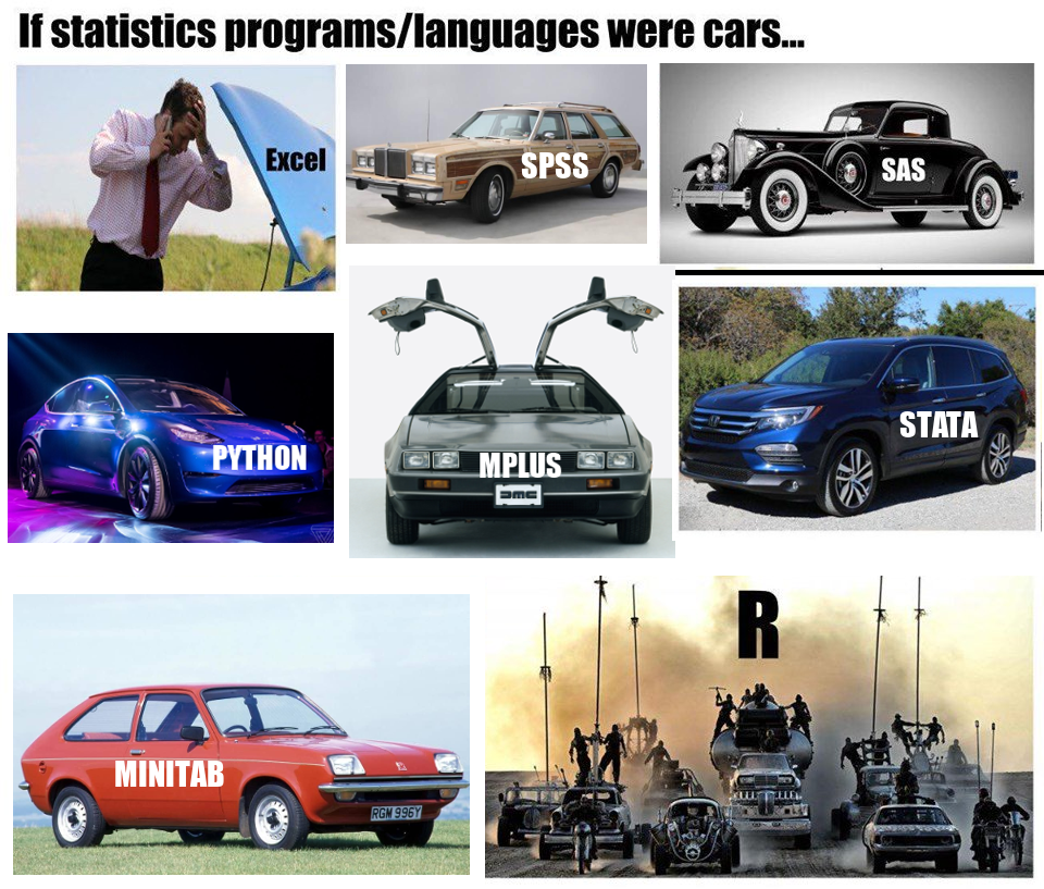
Unlike other statistics programs, R is a free, open source language, and has a very active community committed to programming extensions to R. These extensions are known as libraries, and usually if you have a clear idea of what you want to do in R but can’t find a predefined function to do it, you will find that someone has programmed a library which serves your need. We are grateful to guyjantic on Imgur for visualizing the allure of R over other programs:

 

Introduction to R

This section builds on Gries (2008), chapter 2.

https://uzh.mediaspace.cast.switch.ch/media/0_3eal1bck

In the last chapter, you already got a taste of some simple commands. Here, we briefly recapitulate some of what we discussed in the previous chapter and introduce several more foundational concepts.

For those of you new to programming, it is useful to think of programming as writing sets of calculations and/or commands. These commands have to be entered at the prompt in the console of R. Remember that the prompt is the >.

At the most basic level, we can use R as a calculator. In those cases, we just enter our calculations and get the result:

> 17/2
[1] 8.5

As we have seen, we can also define variables. Variables can take different forms and structures. In addition to numeric data, we often use character strings in linguistics. Character strings are identifiable by the quotation marks around them, as we will see below. Both strings and numerals can come as single values, data frames (which we saw in the last chapter) or vectors, which we discuss at length below.

Here you see an example of a variable which contains a string and of one which contains a numeric vector:

> a<- "Hello World"
> a
[1] "Hello World"
> b=c(1,3,4)
> b
[1] 1 3 4

Note how the strings are identifiable by the quotation marks and the numerals by the absence of quotation marks.

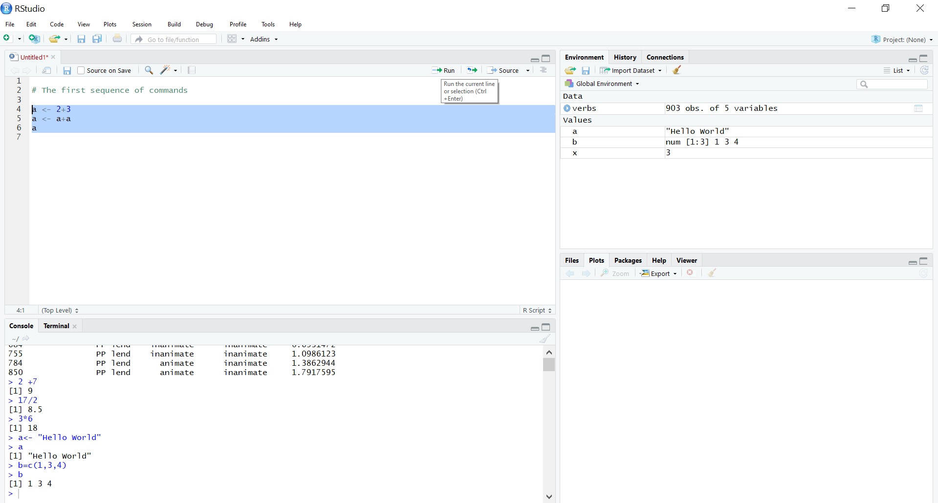
So far, we have only shown examples where there is one command per line. However, it is also possible to enter sequences of commands. To do this, we enter several commands separated by a semicolon:

> a <- 2+3 ; a <- a+a ; a
[1] 10

In RStudio, we can also use the script to write and execute a sequence of commands. When working in the script window of RStudio, you can write each command on a new line. Then you select the lines you want to run and execute them by pressing “Ctrl+Enter” or clicking “Run” in the top right of the window.

As we mentioned above, R contains a lot of predefined functions beyond simple mathematical ones. Unless you use R only as a calculator, you will use functions which take an argument. This means that function is performed on an object, like one of our variables. Let’s begin by looking at a simple mathematical function which takes an argument: the square root. We can use the predefined function sqrt() to calcualte the square root of a numeric value. Let’s overwrite our variable b to become the square root of 5 and then print the result:

> b <- sqrt(5); print(b)
[1] 2.236068

A function we will use a lot is plot(). Let’s a numeric vector to the new variable v and plot the result. The picture below contains the two bottom windows of RStudio, showing the console with the command and the resulting plot.

Another function which takes an argument is sample (). In fact, sample() takes two arguments. Test your intuition of how this function works in the exercise below.

In the last chapter, we already briefly touched on ranges. This is a fairly simple concept, but it can be very useful if you want to generate a bunch of numbers quickly (as sample data, for instance). The operater which enables us to create a range is the :. In the example below, we use this to generate a variable containing a numerical vector ranging from 0 through 10:

> MyRange <- c(0:10) ; MyRange
 [1]  0  1  2  3  4  5  6  7  8  9 10

A final basic concept are indexes, which we also touched on in the last chapter. Indexes refer to particular positions in vectors and can be accessed using square brackets. For instance, to access the fifth position in the MyRange variable, we can use the command:

> MyRange[5]
[1] 4

As we discussed at some length in the last chapter, we can also use indexes to access specific cells in data frames. The data frame examples, of course, had two dimensions (rows and columns), while the vector, being a list, only has one. If you try to incorporate a second dimension in MyRange by inserting a comma in the brackets, you get an error message:

> MyRange[5,]
Error in MyRange[5, ] : incorrect number of dimensions 

 

Sampling and looping

So far, so good, or so we hope. As you might expect, things get more complicated fairly quickly. For instance, we can formulate conditional commands in R, meaning that the output depends on an element which is determined by a step in a squence of commands, rather than by us.

https://uzh.mediaspace.cast.switch.ch/media/0_vijio01q

Take, for example, the sequence of commands below:

> randomthingy = sample(c(1,2,3),1) ; if (randomthingy > 1) {print ("You are lucky")} else {print("I am sorry")}
[1] "You are lucky"

You are now, of course, familiar with the sample() function, so you will immediately see that the first command in this sequence assigns the value 1, 2 or 3 to the variable randomthingy. The second part of the sequence is a little more complicated: it is a logical test. The argument in brackets behind the if, (randomthingy > 1), tests whether the number we sampled before is greater than one. If this is the case, the output is “You are lucky”. If, however, the number we sampled is equal to one, the output is “I am sorry”.

You can see that the conditional output is put in quotation marks, because we want the output to be character strings, and in curly brackets, { }. The curly brackets are referred to as blocks. In this example, the blocks allow us to conditionally define the output.

Blocks are also used in another important feature of programming: loops. Loops allow us to run multiple iterations of a command. Before we discuss what this means in detail, take a look at this example:

> for (i in c(1:3)) {myS = sample(c(1,2,3),i) ; print(myS)}
[1] 2
[1] 2 1
[1] 1 2 3

What is going on here? This is perhaps easiest to grasp by looking at the what is in the block. You can see that it is a squence of familiar commands: in the first, we draw a sample from a vector and assign it to the variable myS, and in the second we tell R to display the variable.

The new element here is the second argument in the sample() function, i. What is i? If you look at the for() command in front of the block, you get the answer. Here, we tell R to iterate through the vector ranging from 1 through 3. This means that in the first iteration, i takes the value 1. Then, the commands in the block are executed. In the second iteration, i takes the value 2. Again, the commands in the block are executed. In the third and final iteration, i takes the value 3. Again, the commands in the block are executed.

If it was slightly repetitive to read the explanation, you have understood why loops are a useful concept. Imagine you want to run a loop through not three, but, say, 10’000 iterations. With this small but powerful line of code, you can sometimes save yourself hours of tedious manual labor.

 

Default assumptions

https://uzh.mediaspace.cast.switch.ch/media/0_oje11hip

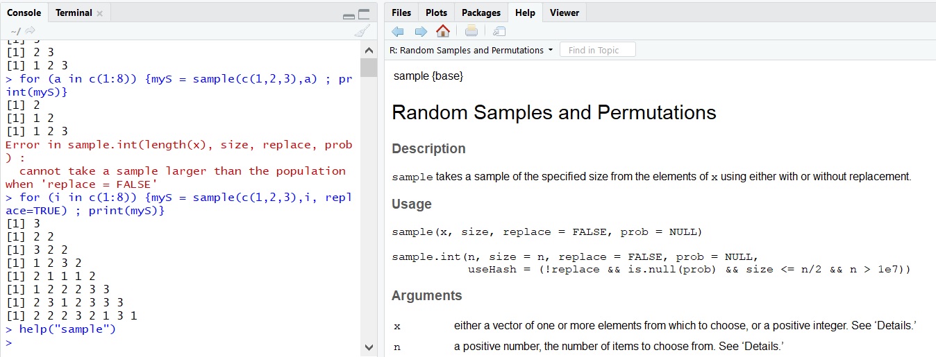
Often it is not entirely clear what a command is supposed to do, and there are many default assumptions being made by R in the background. Run the following loop, which is identical to the one above except that it runs not through three but through eight iterations:

> for (i in c(1:8)) {myS = sample(c(1,2,3),i) ; print(myS)}
[1] 2
[1] 1 2
[1] 1 2 3
Error in sample.int(length(x), size, replace, prob) : 
  cannot take a sample larger than the population when 'replace = FALSE'

The error message R prints shows that we are working with the default assumption under which the sample() function samples without replacement. In other words, there are only three values which can be drawn, and once all three numbers are drawn R prints the error message because it cannot draw the fourth value which would be required in the fourth iteration. In order to avoid this error, we can augment our sample command with a further argument, where we define “replace = TRUE”:

> for (i in c(1:8)) {myS = sample(c(1,2,3),i, replace=TRUE) ; print(myS)}
[1] 3
[1] 2 2
[1] 3 2 2
[1] 1 2 3 2
[1] 2 1 1 1 2
[1] 1 2 2 2 3 3
[1] 2 3 1 2 3 3 3
[1] 2 2 2 3 2 1 3 1

With this additional argument, we allow for sampling with replacement, which means that R can draw each value multiple times. Now the loop runs without error messages.

It is not always obvious which functions take which arguments, let alone what the default assumptions of these arguments are. In those cases, we can look up the default arguments using R’s inbuilt documentation using one of the two help commands: help(sample) or ?sample. If you are using the R base, a new window will open with the documentation file, and if you are using RStudio, the documentation will open in the bottom right window.

In the beginning, the information in the documentation may be more confusing than helpful because of the style it is presented in. Most help pages feature several examples at the end of the page, and it is worth scrolling down to look at those if you get stuck. In time, you will become used to the information in the help pages and understand it readily.

 

Nestedness and assistance

https://uzh.mediaspace.cast.switch.ch/media/0_ycqp6cqk

A further concept we want to introduce is nestedness. Nestedness describes situations where commands contain other commands, leading to a layering of commands. Take a look at the following example:

> sort(sample(c(1,2,3),5, replace=T))
[1] 1 1 2 3 3
> sort(sample(c(1,2,3),5, replace=T))
[1] 1 1 2 2 3

First, let’s focus on the familiar elements. In brackets, we see a sample function which draws 5 observations with replacement from a vector ranging from 1 through 3. We discussed similar examples above, and there we always received an unsorted sample. Here, however, the numbers are sorted in ascending order. You are correct in thinking that this is because of the sort() function. What may be less evident is that we are dealing with nested commands here. You can clearly see this if you perform the steps separately:

> chaos <- sample(c(1,2,3),5, replace=T)
> chaos
[1] 3 1 3 3 3
> order <- sort(chaos)
> order
[1] 1 3 3 3 3

With an example like this, nestedness is fairly easy to see and to work with. However, consider this more complex set of nested elements:

> L <- sample(c(1:10),1); if (L == 1) {print ("O dear ...")} else { if (L > 8) {print("you lucky bastard")}}

It is with examples like this that you will start to get a feeling for the importance of keeping a good overview over your brackets. In the base R, you are responsible for getting the brackets right yourself, while in RStudio offers a bit of assistance on that front by coloring the other half of the bracket grey if your text cursor touches a bracket:

A user-friendly editing function which is included both in RStudio and base R is the history. You can scroll through the history with the “arrow-up” key, which saves you the trouble of copying and pasting if you want to run a command multiple times without (or with few) adjustments. If you scroll back too far, you can use the “arrow-down” key to get to where you want to go. The history allows you to retrieve any command you entered during the current session.

https://uzh.mediaspace.cast.switch.ch/media/0_6hlfnata

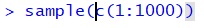
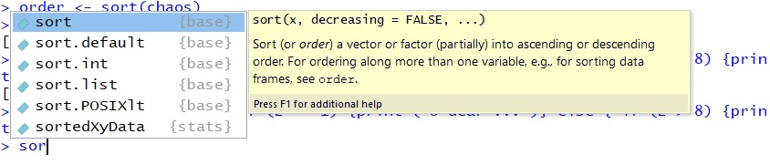
Another user-friendly editing function included in R is the auto-fill. If you type the letters “sor” into the console and hit the TAB key, you will see a small window open which contains all possible completions of “sor”, from sort to sortedXyData. Use the up- and down-arrow keys to navigate through your options and hit TAB again on the one you want.

Armed with these concepts, you should be prepared for most of the things we discuss from here on.

 

Mistakes and the importance of practice

In the beginning, you will make a lot of mistakes. This does not mean anything is wrong with you. From beginners to experienced programmers, everyone makes mistakes and runs into error messages from time to time. In fact, the more time you spend programming, the more error messages you will see. In a sense, learning a programming language forces you to confront your mistakes more than other solitary practices, since computers are extremely nit-picking and take everything you enter exactly as it is, regardless of whether it makes sense or not. To help you avoid more error messages than are necessary, we compiled a list of several frequent mistakes and let you sort out the correct from the incorrect commands.

https://uzh.mediaspace.cast.switch.ch/media/0_c7ry0ht7

You will spend a lot of time browsing manuals, debugging and googling. As the saying goes, there’s no learning like learning the hard way. While this is perhaps a negative way of looking at things, it has a decisively positive flipside: you are in constant interaction with the computer which means it is easy to make progress. So you get error messages, and you get output, and the more you practice, the more often the output will be what you want it to be and at some point you will find solutions to errors more quickly and, eventually, the error messages will become rarer (although if you stop getting any error messages, it means that you probably stopped programming).

What is more, you are not alone in this. The online community has answered a lot of questions, and often it is enough to just google the error message to find a solution. For instance, if you search Google for “R random number generate” you will find many different ways of doing just that. We should also add, though, that it becomes easier to find solutions online if you are familiar with the R terminology, so we would encourage you to think, for example, about “data frames” rather than “tables” when working with R. We cannot practice for you, but we make sure that you pick up the correct terminology from reading this book.

https://uzh.mediaspace.cast.switch.ch/media/0_r1y7v2d8

After our litany on practicing, we want to give one more piece of advice before beginning with statistics proper. One of the difficulties beginners encounter, and indeed some of the most frustrating challenges occur when importing files into R. We already discussed one way of doing that in the previous chapter, where you imported a tab-separated table with headers into R. In addition to tab-separated files, there are two more structures which are worth knowing. Open these two raw text files in new tabs:

vector1.txt and vector2.txt

First of all, since they are one-dimensional we can identify both of these files as vectors. Then, we see that the data points in the first vector are separated with new lines, and those in the second are separated by a whitespace. When importing a file it is very helpful to be aware of how the file is structured.

For instance, if we import vector1.txt using the command we file.choose() that we saw in the previous chapter, we can use a simple piece of code:

> v1 <- scan(file=choose.files())

Again, a window will open and we can open vector1.txt from whereever we saved it. However, if you try to use the same code to open vector2.txt you get an error message:

> v2 <- scan(file=choose.files())
Error in scan(file = choose.files()) : 
  scan() expected 'a real', got 'anton'

The error message occurs for two reasons. Firstly, vector2.txt contains character strings, not numbers. Secondly, the data points are separated, as we said, by a whitespace. We have to augment the scan() command by two arguments:

> v2 <- scan(file=choose.files(),sep=" ",what = "char"); v2
Read 5 items
[1] "anton"  "berta"  "caesar" "dora"   "emil"  

These arguments, which are also called flags, are not optional for the separator and the data type. If you don’t include them, you cannot open vector2.txt.

When working on a script in R over multiple sessions, it becomes tedious to manually select the file you work with each time. In order to target the correct file automatically, adapt the file path and enter the absolute file location:

> v2 <- scan(file="C:/Users/Max/Documents/R/stats for linguistics/chapter 2/vector2.txt", what="char", sep=" ")
Read 5 items

This also works with the read.table() function which we used in the previous chapter:

> verbs <- read.table(file="C:/Users/Max/Documents/R/stats for linguistics/chapter 1/verbs.txt", header=TRUE, sep="\t")

So far, we have only discussed how to get data into R. But, of course, sometimes we want to edit the data in R and then save the results. For this we can use the cat() function.

Imagine, for instance, that you want to create a list of possible names for your unborn child. So far, you have compiled a list of of alphabetically sorted names: the v2 you imported above. You feel that five names just don’t cut it, you want at least seven. So you add the two next candidates to the list:

> v2 <- append(v2, c("friedrich", "gudrun"))

In a next step, you want to save the new variable with seven names so you can print the list and discuss the new additions with your spouse. To do so, you need the cat() function and the arguments it takes: the variable you want to save, the file path and the separator type:

> cat(v2, file="C:/Users/Max/Documents/R/stats for linguistics/chapter 2/vector2_more_names.txt", sep="\n")

Here, we decided to save the longer list as a new file, with line breaks separating the names. If you want to overwrite an existing file, you can also use the file.choose() function:

> cat(v2, file.choose())

 

Vectors

Finally, since we are already working with them, let us add some words about vectors. We have discussed how vectors can be imported, lengthened and saved. With v1 and v2 we have seen that we can store both numeric and character data in vectors. In the example above, we played around with v2, so now let’s take a look at what we can do with the numeric vector, v1.

Like we did above, we can add more information to the vector:

> numbers <- append(v1,c(8,9,11)) ; numbers
[1]  1  2  3  4  5  8  9 11

Then we can calculate the mean:

> mean(numbers)
[1] 5.375

Or run it through a loop:

> for (n in c(1:10)) {numbers = append((mean(numbers)+length(numbers)),numbers)} ; numbers
 [1] 30.65330 28.71213 26.77463 24.84129 22.91272 20.98965 19.07298 17.16389 15.26389 13.37500  1.00000
[12]  2.00000  3.00000  4.00000  5.00000  8.00000  9.00000 11.00000

There are many ways to manipulate numeric vectors, and we will discuss them more in subsequent chapters.

What happens if we encounter a vector which contains both numbers and words? We can try that out by generating one:

> a <- c(1,2,3, "hi!")

First, let’s check whether this is even a vector:

> is.vector(a)
[1] TRUE

We can also check out whether a has as many positions as we think it does:

> length(a)
[1] 4

Then, we can use the str() function to view the structure of this object a:

> str(a)
 chr [1:4] "1" "2" "3" "hi!"

Here, we see that even the numbers in this vector are characters. This makes sense since R is incapable of coercing characters strings into numbers:

> as.integer(a)
[1]  1  2  3 NA
Warning message:
NAs introduced by coercion 

And since numbers can be converted into characters, this is what R does.

Use your understanding of how vectors to build a simple random name generator:

In the next couple of chapters, we will discuss the fundamentals of statistics, which means we will be working mostly with numeric data. Find out what this means in detail by continuing to the next chapter, Basics of Descriptive Statistics.

 

If you are interested in acquainting yourself with further useful functions in R before continuing, we recommend reading the documentation of and playing around with the following functions:

• as.characters
• as.integers
• attach
• plot
• hist
• barplot
• pie

For further reading and more exercises we recommend reading chapter 2 in Gries (2008) and visiting his website at http://www.stgries.info/research/sflwr/sflwr.html.

 

Reference:

Gries, Stefan Th. 2008. Statistik für Sprachwissenschaftler. Göttingen: Vandenhoeck & Ruprecht.